Abstracts - KTH Mechanics

Coupling weather-scale flow with street scale computations
Zhengtong Xie ∗ and Ian P. Castro ∗
Understanding the mechanisms by which the urban boundary layer and regional
weather are coupled aerodynamically and thermodynamically is known to be vital
but is still in its infancy. For the former, unsteadiness of a large scale (periodic)
driving flow is known to have a significant impact on the turbulent flows 1 . One might
anticipate similar effects in the urban boundary layer. For the latter, one could note
that the temperature in cities has been found to be up to ten degrees higher than the
surrounding rural areas and to cause large increases in rainfall amounts downwind 2 .
In operational regional weather models the horizontal grid is no less than 1km, which
eliminates most of the turbulent fluctuations. To investigate turbulent flows in an
urban area down to a resolution one meter, small-scale computational fluid dynamics
will inevitably have to be applied. Our objective is to develop tools for implementing
unsteady spatial boundary conditions derived from the output of much larger-scale
computations (UK Met Office’s Unified Model) with a large-eddy simulation code
for computing the street-scale flow. Flow over groups of cubes mounted on a wall
provides an excellent test case for validation of LES. In order to avoid massive precursor
computation, an efficient quasi-steady inlet condition has been developed and
implemented with carefully designed artificially imposed turbulence fluctuations with
prescribed integral length scales and intensities.
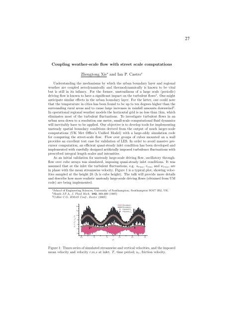
As an initial validation for unsteady large-scale driving flow, oscillatory throughflow
over cube arrays was simulated, imposing quasi-steady inlet conditions. It was
assumed that at the inlet the turbulent fluctuations, e.g. urms, vrms and wrms, are
in phase with the mean streamwise velocity. Figure 1 is a typical plot, showing velocities
sampled at the height 2h (h is cube height). The talk will provide more details
and describe how more realistic unsteady large-scale driving flows (obtained from UM
code) are being implemented.
∗ School of Engineering Sciences, University of Southampton, Southampton SO17 1BJ, UK.
1 Sleath J.F.A, J. Fluid Mech. 182, 369-409 (1987)
2 Collier C.G. RMetS Conf., Exeter (2005)
(u, v, U m , u rms )/u *
20
16
12
8
4
0
-4
0.5 1.0 1.5 2.0 2.5 3.0
t/T
Simulated v
Simulated u
Imposed U m
Imposed u rms
Figure 1: Times series of simulated streamwise and vertical velocities, and the imposed
mean velocity and velocity r.m.s at inlet. T , time period; u∗, friction velocity.
27