Abstracts - KTH Mechanics

52
The Parabolised Stability Equations for 3D-Flows:
Implementation and Numerical Stability
M. S. Broadhurst ∗ ,S.J.Sherwin ∗
The numerical implementation of the parabolised stability equations (3D-PSE)
using a substructuring solver - designed to take advantage of a spectral/hp-element
discretisation - is considered. Analogous to the primitive variable form of the twodimensional
PSE 1 , the equations are ill-posed 2 ; although choosing an Euler implicit
scheme in the streamwise z-direction yields a stable scheme for sufficiently large step
∂ ˆp
sizes (∆z >1/|β|, whereβis the streamwise wavenumber). Neglecting the ∂z term
relaxes the lower limit on the step-size restriction. The θ-scheme is also considered,
and the step-size restriction is determined. Neglecting the pressure gradient term
shows stable eigenspectra for θ ≥ 0.5. For θ = 0.5, the formulation corresponds to the
second order Cranck-Nicholson scheme. Consequently, for identical step-sizes in the
streamwise direction, the truncation error will be lower than the Euler implicit scheme,
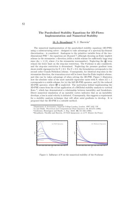
and this can be taken advantage of when solving the 3D-PSE. Figure 1 illustrates
how the absolute value of the most unstable eigenvalue varies with θ, where|G| < 1
corresponds to a stable scheme, for (a) the full 3D-PSE operator, and (b) the reduced
∂ ˆp
3D-PSE operator, where ∂z is neglected. The motivation behind implementing the
3D-PSE comes from the recent application of a BiGlobal stability analysis to vortical
flows 3 , which has demonstrated a relationship between instability and breakdown.
Direct numerical simulation of an unstable vortex indicates that as an instability
develops, a loss in axial velocity is initiated. Consequently, this suggests a requirement
for a stability analysis technique that will allow axial gradients to develop. It is
proposed that the 3D-PSE is a suitable method.
∗ Department of Aeronautics, Imperial College London, London. SW7 2AZ. UK
1 LiandMalik, Theoretical and Computational Fluid Dynamics. 8, 253-273 (1996).
2 Andersson, Henningson and Hanifi, J. Eng. Math. 33, 311-332 (1998).
3 Broadhurst, Theofilis and Sherwin, IUTAM Symposium on LTT. Kluwer (In Press).
max|G|
10
∆z =0.4
9
8
7
6
∆z =0.3
5
4
∆z =0.2
3
2 ∆z =0.1
1
(a) Full Operator
9
8
(b) Reduced Operator
0
0 0.1 0.2 0.3 0.4 0.5
θ
0.6 0.7 0.8 0.9 1
max|G|
10
7
6
5
4
3
2
1
0
0 0.1 0.2 0.3 0.4 0.5
θ
0.6 0.7 0.8 0.9 1
Figure 1: Influence of θ on the numerical stability of the θ-scheme