Alma Mater Studiorum Universit`a degli Studi di Bologna ... - Inaf
Alma Mater Studiorum Universit`a degli Studi di Bologna ... - Inaf
Alma Mater Studiorum Universit`a degli Studi di Bologna ... - Inaf

You also want an ePaper? Increase the reach of your titles
YUMPU automatically turns print PDFs into web optimized ePapers that Google loves.
4.6. Three-<strong>di</strong>mensional analysis 59<br />
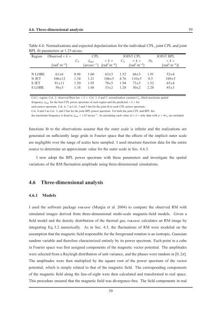
Table 4.4: Normalizations and expected depolarization for the in<strong>di</strong>vidual CPL, joint CPL and joint<br />
BPL fit parameters at 1.25 arcsec.<br />
Region Observed< k> CPL JOINT CPL JOINT BPL<br />
C 0 f max < k> C 0 < k> D 0 < k><br />
[rad 2 m −4 ] [arcsec −1 ] [rad 2 m −4 ] [rad 2 m −4 ] [rad 2 m −4 )]<br />
N LOBE 61±6 0.96 1.60 63±3 1.52 66±3 1.91 52±4<br />
N JET 106±12 1.34 1.21 106±5 4.76 110±5 0.5 109±5<br />
S JET 91±11 1.50 1.95 70±5 1.94 73±5 1.52 65±4<br />
S LOBE 50±5 1.18 1.68 53±2 1.28 50±2 2.20 45±3<br />
Col.1: region; Col. 2: observed Burn law< k>. Col. 3, 4 and 5: normalization constant C 0 , fitted maximum spatial<br />
frequency f max for the best CPL power spectrum of each region and the pre<strong>di</strong>cted for<br />
each power spectrum. Col. 6, 7 as Col. 3 and 5 but for the joint fit to each CPL power spectrum;<br />
Col. 8 and 9 as Col. 3, and 5 but for the joint BPL power spectrum. For both the joint CPL and BPL fits,<br />
the maximum frequency is fixed at f max = 1.67 arcsec −1 . In calculating each value of< k> only data with p>4σ p are included.<br />
functions fit to the observations assume that the outer scale is infinite and the realizations are<br />
generated on sufficiently large grids in Fourier space that the effects of the implicit outer scale<br />
are negligible over the range of scales here sampled. I used structure-function data for the entire<br />
source to determine an approximate value for the outer scale in Sec. 4.6.3.<br />
I now adopt the BPL power spectrum with these parameters and investigate the spatial<br />
variations of the RM fluctuation amplitude using three-<strong>di</strong>mensional simulations.<br />
4.6 Three-<strong>di</strong>mensional analysis<br />
4.6.1 Models<br />
I used the software packageFARADAY (Murgia et al. 2004) to compare the observed RM with<br />
simulated images derived from three-<strong>di</strong>mensional multi-scale magnetic-field models. Given a<br />
field model and the density <strong>di</strong>stribution of the thermal gas,FARADAY calculates an RM image by<br />
integrating Eq. 3.2 numerically. As in Sec. 4.5, the fluctuations of RM were modeled on the<br />
assumption that the magnetic field responsible for the foreground rotation is an isotropic, Gaussian<br />
random variable and therefore characterized entirely by its power spectrum. Each point in a cube<br />
in Fourier space was first assigned components of the magnetic vector potential. The amplitudes<br />
were selected from a Rayleigh <strong>di</strong>stribution of unit variance, and the phases were random in [0, 2π].<br />
The amplitudes were then multiplied by the square root of the power spectrum of the vector<br />
potential, which is simply related to that of the magnetic field. The correspon<strong>di</strong>ng components<br />
of the magnetic field along the line-of-sight were then calculated and transformed to real space.<br />
This procedure ensured that the magnetic field was <strong>di</strong>vergence-free. The field components in real<br />
59