Alma Mater Studiorum Universit`a degli Studi di Bologna ... - Inaf

4.6. Three-dimensional analysis 61
number of simulations for each combination of field strength and radial profile and to compare
the predicted and observed values ofσ RM evaluated over the boxes used in Sec. 4.3.1 (Fig. 4.2). I
usedχ 2 summed over the boxes as a measure of the goodness of fit. This procedure is independent
of the precise value of the outer scale, provided that it is much larger than the averaging boxes. I
express the results in terms ofχ 2 red , which is the value ofχ2 divided by the number of degrees of
freedom.
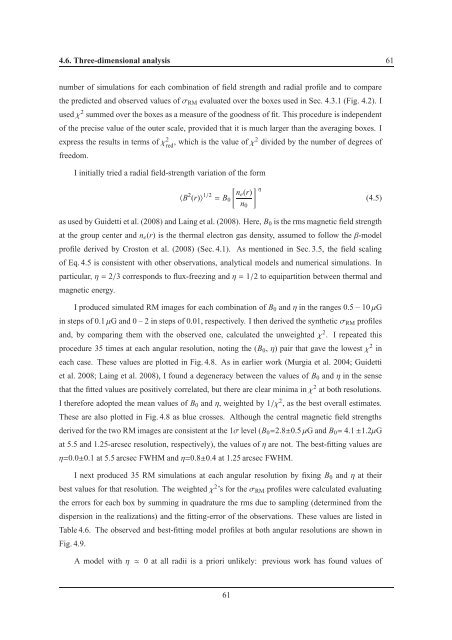
I initially tried a radial field-strength variation of the form
〈B 2 (r)〉 1/2 = B 0
[
ne (r)
n 0
] η
(4.5)
as used by Guidetti et al. (2008) and Laing et al. (2008). Here, B 0 is the rms magnetic field strength
at the group center and n e (r) is the thermal electron gas density, assumed to follow theβ-model
profile derived by Croston et al. (2008) (Sec. 4.1). As mentioned in Sec. 3.5, the field scaling
of Eq. 4.5 is consistent with other observations, analytical models and numerical simulations. In
particular,η=2/3 corresponds to flux-freezing andη=1/2 to equipartition between thermal and
magnetic energy.
I produced simulated RM images for each combination of B 0 andηin the ranges 0.5 – 10µG
in steps of 0.1µG and 0 – 2 in steps of 0.01, respectively. I then derived the syntheticσ RM profiles
and, by comparing them with the observed one, calculated the unweightedχ 2 . I repeated this
procedure 35 times at each angular resolution, noting the (B 0 ,η) pair that gave the lowestχ 2 in
each case. These values are plotted in Fig. 4.8. As in earlier work (Murgia et al. 2004; Guidetti
et al. 2008; Laing et al. 2008), I found a degeneracy between the values of B 0 andηin the sense
that the fitted values are positively correlated, but there are clear minima inχ 2 at both resolutions.
I therefore adopted the mean values of B 0 andη, weighted by 1/χ 2 , as the best overall estimates.
These are also plotted in Fig. 4.8 as blue crosses. Although the central magnetic field strengths
derived for the two RM images are consistent at the 1σ level (B 0 =2.8±0.5µG and B 0 = 4.1±1.2µG
at 5.5 and 1.25-arcsec resolution, respectively), the values ofηare not. The best-fitting values are
η=0.0±0.1 at 5.5 arcsec FWHM andη=0.8±0.4 at 1.25 arcsec FWHM.
I next produced 35 RM simulations at each angular resolution by fixing B 0 andηat their
best values for that resolution. The weightedχ 2 ’s for theσ RM profiles were calculated evaluating
the errors for each box by summing in quadrature the rms due to sampling (determined from the
dispersion in the realizations) and the fitting-error of the observations. These values are listed in
Table 4.6. The observed and best-fitting model profiles at both angular resolutions are shown in
Fig. 4.9.
A model withη ≃ 0 at all radii is a priori unlikely: previous work has found values of
61