Mass and Light distributions in Clusters of Galaxies - Henry A ...

WL Determination of the Distance-Redshift Relation
1
0.9
0.8
0.7
χ 2 /dof = 19/8
0.6
g T
0.5
0.4
0.3
0.2
0.1
0
1 2 5 10
θ [arcmin]
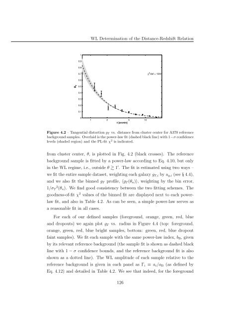
Figure 4.2 – Tangential distortion g T vs. distance from cluster center for A370 reference
background samples. Overlaid is the power-law fit (dashed black line) with 1−σ confidence
levels (shaded region) and the PL-fit χ 2 is indicated.
from cluster center, θ, is plotted in Fig. 4.2 (black crosses). The reference
background sample is fitted by a power-law according to Eq. 4.10, but only
in the WL regime, i.e., outside θ 1 ′ . The fit is estimated using two ways –
we fit the entire sample dataset, weighting each galaxy g T,i by u g,i (see § 4.4),
and we also fit the binned g T profile, 〈g T (θ n )〉, weighting by the bin error,
1/σ 2 T (θ n ). We find good consistency between the two fitting schemes. The
goodness-of-fit χ 2 values of the binned fit are displayed next to each powerlaw
fit, and also in Table 4.2. As can be seen, a simple power-law serves as
a reasonable fit in all cases.
For each of our defined samples (foreground, orange, green, red, blue
and dropouts) we again plot g T vs. radius in Figure 4.4 (top: foreground,
orange, green, red, blue bright samples, bottom: green, red, blue dropout
faint samples). We fit each sample with the same power-law index, b B , given
by its relevant reference background (the sample fit is shown as dashed black
line with 1 − σ confidence bounds, and the reference background fit is also
shown as a dotted line). The WL amplitude of each sample relative to the
reference background is given in each panel as Γ i ≡ a i /a B (as defined by
Eq. 4.12) and detailed in Table 4.2. We see that indeed, for the foreground
126