Mass and Light distributions in Clusters of Galaxies - Henry A ...

Weak Lensing Dilution in A1689
0.85
0.8
0.75
1.4
1.3
1.2
1.1
0.696
0.694
0.692
0.69
0.78
0.77
0.76
0.75
1.95
1.9
1.85
24.5 25 25.5 26 26.5 27
Limiting magnitude
0.849
0.846
0.843
0.84
24.5 25 25.5 26 26.5 27
Limiting magnitude
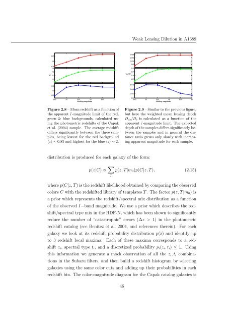
Figure 2.8 – Mean redshift as a function of
the apparent i’-magnitude limit of the red,
green & blue backgrounds, calculated using
the photometric redshifts of the Capak
et al. (2004) sample. The average redshift
differs significantly between the three samples,
being lowest for the red background
〈z〉 ∼ 0.85 and highest for the blue 〈z〉 ∼ 2.
Figure 2.9 – Similar to the previous figure,
but here the weighted mean lensing depth
D ds /D s is calculated as a function of the
apparent i’-magnitude limit. The expected
depth of the samples differs significantly between
the samples and in general the distance
ratio grows only slowly with increasing
apparent magnitude for each sample.
distribution is produced for each galaxy of the form:
p(z|C) ∝ ∑ T
p(z, T |m 0 )p(C|z, T ), (2.15)
where p(C|z, T ) is the redshift likelihood obtained by comparing the observed
colors C with the redshifted library of templates T . The factor p(z, T |m 0 ) is
a prior which represents the redshift/spectral mix distribution as a function
of the observed I−band magnitude. We use a prior which describes the redshift/spectral
type mix in the HDF-N, which has been shown to significantly
reduce the number of “catastrophic” errors (∆z > 1) in the photometric
redshift catalog (see Benítez et al. 2004, and references therein). For each
galaxy we look at its redshift probability distribution p(z) and identify up
to 3 redshift local maxima. Each of these maxima corresponds to a redshift
z i , spectral type t i , and a discretized probability p i (z i , t i ) ≤ 1. Using
this information we generate a mock observation of all the z i , t i combinations
in the Subaru filters, and then build a redshift histogram by selecting
galaxies using the same color cuts and adding up their probabilities in each
redshift bin. The color-magnitude diagram for the Capak catalog galaxies is
46