Mass and Light distributions in Clusters of Galaxies - Henry A ...

Weak Lensing Dilution in A1689
g +
−1
0’−1’, ACS
0.2
−1.05
1’−2’, ACS
0.1
2’−4’, Subaru
−1.1 α
0
10 3 4’−8’, Subaru −1.15
α=−1.046 M *
=−21.46
−1
0.3
−1.05
g +
0.2
0.1
−1.1 α
0
10 2
−1.15
α=−1.059 M *
=−20.77
−1
0.08
g + 0.04
−1.05
−1.1 α
−1.15
0
10 1
α=−1.094 M *
=−21.21
0.06
−1
0.04
−1.05
g +
−1.1
0.02
α
−1.15
0
10 0
α=−1.108 M *
=−21.41
−24 −22 −20 −18 −16 −14 −12 −24 −22 −20 −18 −16 −14 −12 −23 −22 −21 −20
M i’
M i’
M *i’
Φ(M) [h 2 Mpc −2 mag −1 ]
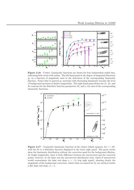
Figure 2.16 – Center: Luminosity functions are shown for four independent radial bins,
indicating little trend with radius. The left-hand panel is the degree of tangential distortion
g T as a function of magnitude used in the derivation of the corresponding luminosity
function. Notice that in general g T increases with decreasing luminosity because the level
of background increases at fainter magnitudes. The right-hand panel shows the 1σ, 2σ, and
3σ contours for the Schechter function parameters M ∗ and α, for each of the corresponding
luminosity functions.
10 3 uncorrected
corrected
−10 0.151
10 2
−10 0.152
Φ(M) [h 2 Mpc −2 mag −1 ]
10 1
10 0
10 −1
uncorrected, α=−1.421
M i’
−10 0.153
−1
−1.02
−1.04
α
−1.06
−1.08
10 −2
−24 −22 −20 −18 −16 −14
M i’
corrected, α=−1.048
−24 −22
M i’*
−20 −1.1
Figure 2.17 – Composite luminosity function of the cluster (black squares), for r < 10 ′ ,
with the fit to a Schechter function displayed in the lower right panel. The green circles
show the luminosity distribution without the correction made for the background dilution.
At bright magnitudes, there is little difference between the uncorrected and the corrected
points, however, at the faint end the uncorrected distribution rises, which if uncorrected
would overestimate the faint end slope α ∼ 1.4 (top right panel), showing clearly the
magnitude of the background correction, which when accounted for by our method results
a flat faint end slope, α ∼ 1.