10 - H1 - Desy

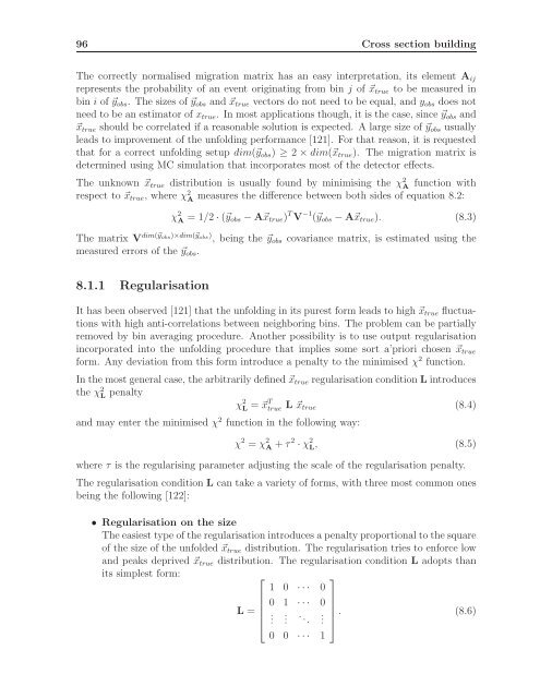
96 Cross section building
The correctly normalised migration matrix has an easy interpretation, its element A ij
represents the probability of an event originating from bin j of ⃗x true to be measured in
bin i of ⃗y obs . The sizes of ⃗y obs and ⃗x true vectors do not need to be equal, and y obs does not
need to be an estimator of x true . In most applications though, it is the case, since ⃗y obs and
⃗x true should be correlated if a reasonable solution is expected. A large size of ⃗y obs usually
leads to improvement of the unfolding performance [121]. For that reason, it is requested
that for a correct unfolding setup dim(⃗y obs ) ≥ 2 × dim(⃗x true ). The migration matrix is
determined using MC simulation that incorporates most of the detector effects.
The unknown ⃗x true distribution is usually found by minimising the χ 2 A function with
respect to ⃗x true , where χ 2 A measures the difference between both sides of equation 8.2:
χ 2 A = 1/2 · (⃗y obs − A⃗x true ) T V −1 (⃗y obs − A⃗x true ). (8.3)
The matrix V dim(⃗y obs)×dim(⃗y obs ) , being the ⃗y obs covariance matrix, is estimated using the
measured errors of the ⃗y obs .
8.1.1 Regularisation
It has been observed [121] that the unfolding in its purest form leads to high ⃗x true fluctuations
with high anti-correlations between neighboring bins. The problem can be partially
removed by bin averaging procedure. Another possibility is to use output regularisation
incorporated into the unfolding procedure that implies some sort a’priori chosen ⃗x true
form. Any deviation from this form introduce a penalty to the minimised χ 2 function.
In the most general case, the arbitrarily defined ⃗x true regularisation condition L introduces
the χ 2 L penalty χ 2 L = ⃗xT true L ⃗x true (8.4)
and may enter the minimised χ 2 function in the following way:
χ 2 = χ 2 A + τ2 · χ 2 L , (8.5)
where τ is the regularising parameter adjusting the scale of the regularisation penalty.
The regularisation condition L can take a variety of forms, with three most common ones
being the following [122]:
• Regularisation on the size
The easiest type of the regularisation introduces a penalty proportional to the square
of the size of the unfolded ⃗x true distribution. The regularisation tries to enforce low
and peaks deprived ⃗x true distribution. The regularisation condition L adopts than
its simplest form:
⎡ ⎤
1 0 · · · 0
0 1 · · · 0
L =
⎢ .
⎣ . . .. ⎥ . ⎦ . (8.6)
0 0 · · · 1