10 - H1 - Desy

18 Theoretical framework
e
e
e
a) b)
γ
e
g
γ
p
p
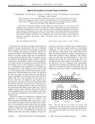
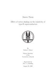
Figure 1.14: Examples for the fragmentation process at LO (a) and NLO (b).
Following the distinction above, the prompt photon cross section can be divided into
four parts: direct non-fragmentation σ nonfrag
dir
, direct fragmentation σ frag
dir
, resolved nonfragmentation
σres
nonfrag and resolved fragmentation σres
frag and factorised in the following
way:
dσ nonfrag
dir
= ∑ f a/p (x, µ 2 ) ⊗ f γ/e (y) ⊗ σ aγ→γX , (1.33)
dσ frag
dir
= ∑ f a/p (x, µ 2 ) ⊗ f γ/e (y) ⊗ σ aγ→dX ⊗ D γ/d (z), (1.34)
dσ nonfrag
res = ∑ f a/p (x, µ 2 ) ⊗ f γ/e (y) ⊗ f b/γ (x γ , µ 2 ) ⊗ σ ab→γX , (1.35)
dσ frag
res = ∑ f a/p (x, µ 2 ) ⊗ f γ/e (y) ⊗ f b/γ (x γ , µ 2 ) ⊗ σ aγ→dX ⊗ D γ/d (z). (1.36)
Here, f a/p (x, µ 2 ) and f b/γ (x γ , µ 2 ) is the already introduced probability of finding parton
a in a proton and a photon respectively given longitudinal momentum fraction x and a
scale probing the partonic structure µ. Similarly, f γ/e (y) is the photon flux calculated
with the Weiszäcker-Williams approximation (see equation 1.28). D γ/d (z) describes the
fragmentation of the parton into the photon.
The parton fragmentation function D γ/d (z) gives the probability that the parton d will
produce a photon γ carrying a fraction z of the parton momentum. It should be noted
that already at leading order a collinear singularity appears in the photon emission by the
quark. As physical cross sections are necessarily finite, the singularity may be factorised
into the fragmentation function defined at the factorisation scale µ F,γ . Within the so-called
phase space slicing method [33] a parameter y min can be introduced, which separates the
divergent collinear contribution from the finite contribution, where the outgoing quark and
photon are still theoretically resolved. In this context the quark-to-photon fragmentation
function at order α is given by [34]:
D γ/d (z) = D γ/d (z, µ F,γ ) + αe2 q
2π
(
P (0)
qγ (z) ln z(1 − z)y mins eq
µ 2 F,γ
+ z
)
, (1.37)
where D γ/d (z, µ F,γ ) describes the non perturbative transition q → γ at the factorisation
scale µ F,γ . The second term represents the finite part after absorption of the collinear
quark-photon contribution into the bare fragmentation function separated by the parameter
y min . The variable e q denotes the charge of quark q and s eq the electron-quark centre of