10 - H1 - Desy

118 Cross section building
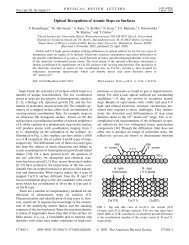
The double dimensional E γ T − ηγ distribution of original MC set I and a f toy
E T ,η
reweighted MC is presented in the figure 8.10.
Entries
150
100
Entries
150
100
50
50
0
-1
0
γ
η
1
2
14
12
γ
E T
10
8
[GeV]
6
0
-1
0
γ
η
1
2
14
12
γ
E T
10
8
[GeV]
6
Figure 8.10: The E γ T -ηγ distribution of the original MC set I and a MC reweighted with
the f toy
E T ,η function.
8.6.1 Fitting procedure
The quality of the whole unfolding procedure is additionally verified by using an alternative
method of cross section determination. The method explained below was used to
determine the prompt photon cross sections in most of the prompt photon publications
based on the HERA data (i.e. [43], [35]) combines the discriminator fitting with bin-to-bin
acceptance correction.
In this method, the discriminator D (see section 6.3) is binned in the transverse energy
E γ T and pseudorapidity ηγ of the photon in bins directly corresponding to the binning
used for the output. In the case of this analysis, that corresponds to twenty bins of
4(E γ T,OUT4 ) × 5(ηγ OUT5
) grid with the actual bin edges listed in appendix table A-4. A
similar grid is filled using pure signal MC and pure background MC. In every bin i the
actual amount of prompt photon signal is extracted using independent minimal-χ 2 fit of
the normalised signal (d sig ) and background (d bkg ) discriminator distributions to the data.
The χ 2 D function is defined as
χ 2 D(N sig,i , N bkg,i ) = ∑ j
(N data,i,j − N bkg,i d bkg,j − N sig,i d sig,j ) 2
σ 2 data,i,j + N2 bkg,i σ2 bkg,j + N2 sig,i σ2 sig,j
(8.46)
where σ data , σ sig and σ bkg are the data, signal and background errors, N sig and N bkg are
parameters representing fitted number of signal and background events and the sum runs