Transportation Spending by Low-Income California Households ...

More documents

Recommendations

Info

household level than taking the average of transportation expenditures and dividing <strong>by</strong> the average of total household expenditures. 154
Appendix D Methods Used for the Example Commute Analysis We used the following steps to identify and cost out the illustrative commutes for Chapter 4. 1. Identify the origins of the commutes. a. Use CTPP data to identify two neighborhoods (TAZs) in each county with the highest number of low-income residents. b. Use ArcGIS software to identify the geographic centroid of each low-income TAZ polygon as the exact point to use for the origin of the commute. 2. Identify the destinations of the commutes: a. Use PUMS data to identify the most common place of work (county) for low-income workers who work outside their county of residence. 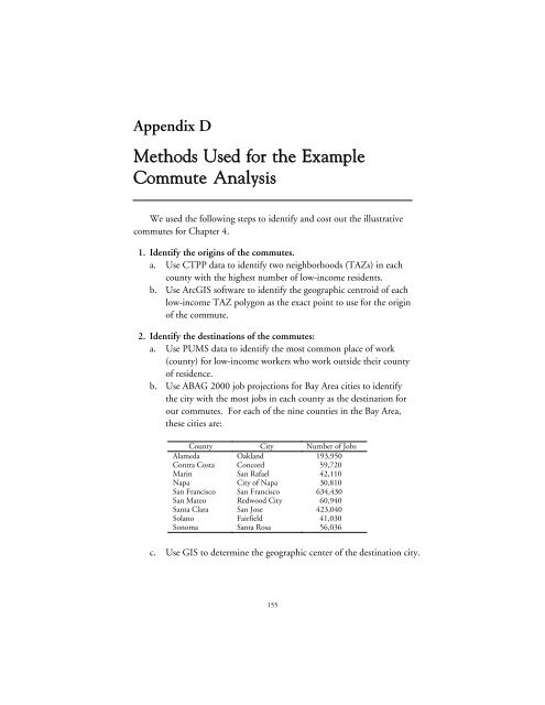b. Use ABAG 2000 job projections for Bay Area cities to identify the city with the most jobs in each county as the destination for our commutes. For each of the nine counties in the Bay Area, these cities are: County City Number of Jobs Alameda Oakland 193,950 Contra Costa Concord 59,720 Marin San Rafael 42,110 Napa City of Napa 30,810 San Francisco San Francisco 634,430 San Mateo Redwood City 60,940 Santa Clara San Jose 423,040 Solano Fairfield 41,030 Sonoma Santa Rosa 56,036 c. Use GIS to determine the geographic center of the destination city. 155
Page 1 and 2:
Transportation Spending by Low-Inco
Page 3 and 4:
Foreword Mismatches between jobs an
Page 5 and 6:
Summary Transportation is an import
Page 7 and 8:
Table S.1 Median Annual Transportat
Page 9 and 10:
about 5 to 10 percent of the median
Page 11:
providing discounted transit fares
Page 14 and 15:
5. COMMUTE BEHAVIOR IN THE BAY AREA
Page 17:
Figures S.1. Vehicle Ownership and
Page 20 and 21:
4.3. Costs of Illustrative Within-C
Page 23 and 24:
1. Introduction Costs associated wi
Page 25 and 26:
of “welfare-to-work” transporta
Page 27:
lays out policy options for address
Page 31 and 32:
2. Data and Methods In this report,
Page 33 and 34:
advantage to this approach is that
Page 35 and 36:
3. Transportation Expenditures in M
Page 37 and 38:
Table 3.2 Vehicle Use, Vehicle Owne
Page 39 and 40:
Components of Vehicle-Related Expen
Page 41 and 42:
inspection, and auto club membershi
Page 43 and 44:
income households and the higher-in
Page 45 and 46:
eport looks primarily at cost and n
Page 47 and 48:
The results from Table 3.5 indicate
Page 49 and 50:
variation in transportation costs w
Page 51 and 52:
overall household expenditures for
Page 53 and 54:
31 Table 3.9 Transportation Expendi
Page 55 and 56:
Table 3.10 Comparison of California
Page 57 and 58:
Table 3.11 Comparison of the San Fr
Page 59 and 60:
Table 3.10 have lower expenditure f
Page 61 and 62:
4. Costs of Illustrative Bay Area C
Page 63 and 64:
0-300 301-600 601-1100 1101-6813 Ba
Page 65 and 66:
Table 4.2 Place of Work Comparison
Page 67 and 68:
Concord CONTRA COSTA SAN FRANCISCO
Page 69 and 70:
Administration (FHWA) mileage rate
Page 71 and 72:
49 Table 4.3 Costs of Illustrative
Page 73 and 74:
participants who took transit or ca
Page 75 and 76:
Table 4.4 Costs of Illustrative Wit
Page 77 and 78:
Page 79 and 80:
Page 81 and 82:
commutes is $4,240, whereas the hig
Page 83 and 84:
The results from this chapter seem
Page 85 and 86:
5. Commute Behavior in the Bay Area
Page 87 and 88:
We also looked at mode choice using
Page 89 and 90:
longer for higher-income workers if
Page 91 and 92:
Table 5.3 (continued) Low- Income H
Page 93 and 94:
Table 5.5 depicts the share of the
Page 95 and 96:
73 Table 5.6 Mode Choice and Vehicl
Page 97 and 98:
75 Table 5.8 Mode Choice and Vehicl
Page 99 and 100:
households report having access to
Page 101 and 102:
Table 5.9 (continued) % Using Each
Page 103 and 104:
• Marin to San Francisco: As with
Page 105 and 106:
Table 5.10 Median Commute Durations
Page 107 and 108:
85 Table 5.11 Differences in Mode C
Page 109 and 110:
Table 5.13 Mode Choice, Work Schedu
Page 111:
trips, make more household-supporti
Page 114 and 115:
only expenditures. Paying a given n
Page 116 and 117:
improving service quality rather th
Page 119:
Part II Policy Strategies and Areas
Page 122 and 123:
potential social costs such as poll
Page 124 and 125:
• Increasing income directly, to
Page 126 and 127: grants for developments that meet c
Page 128 and 129: make it easier for various entities
Page 130 and 131: pass.” 10 Perhaps discounts could
Page 132 and 133: free transit is most likely not app
Page 134 and 135: have fares based on the time of day
Page 136 and 137: hours for late night and graveyard
Page 138 and 139: credit ratings, assisting with insu
Page 140 and 141: would have paid with traditional au
Page 142 and 143: citizens. Rather, the question shou
Page 144 and 145: Facilitating Bicycling or Walking A
Page 146 and 147: transportation hubs may be another
Page 148 and 149: allowing flexibility at the local l
Page 150 and 151: services, health care, drug treatme
Page 152 and 153: costs. Efforts to incorporate infor
Page 154 and 155: are differences) and by looking at
Page 156 and 157: Dataset Poor Low-Income Higher-Inco
Page 158 and 159: income, problems common to most hou
Page 160 and 161: or the Bay Area specifically. We us
Page 163 and 164: Appendix B Information on Specific
Page 165 and 166: We also excluded expenditures on bi
Page 167 and 168: Atlanta: Atlanta, GA MSA Miami: Mia
Page 169 and 170: 147 Table B.1 (continued) CES Metro
Page 171 and 172: Appendix C Sensitivity Analysis for
Page 173 and 174: 151 Table C.1 (continued) Poor Low-
Page 175: transportation expenditures constit
Page 179 and 180: Bibliography American Automobile As
Page 181 and 182: Implications of Welfare Reform for
Page 183 and 184: Lucas, M., and C. Nicholson, “Sub
Page 185 and 186: Progressive Casualty Insurance Comp
Page 187: About the Author LORIEN RICE Lorien
show all

Transportation Spending by Low-Income California Households ...

Create successful ePaper yourself

Delete template?

Save as template?