principles and applications of microearthquake networks

2.2. Central California Microearthquake Network 25
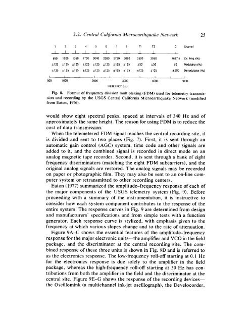
1 2 3 4 5 6 7 8 T1 T2 C Channel
I I I I I I 1 I 1 1 I
680 1020 1360 1700 2040 2380 2720 3060 3500 3950 46875 Ctr Freq (HI)
+I25 k125 k125 f125 i125 i125 +125 2125 f50 k50 k0 Modulation (Hz)
k125 i125 +125 f125 f125 f125 k125 2125 z125 f125 +ZOO Derodulation (Hz)
I I 1 I I I I I I 1
500 1000 2000 3000 4000 5000
FREOUENCY (Hz)
Fig. 8. Format of frequency division multiplexing (FDM) used for telemetry transmission
and recording by the USGS Central California Microearthquake Network (modified
from Eaton, 1976).
would show eight spectral peaks, spaced at intervals of 340 Hz and of
approximately the same height. The reason for using FDM is to reduce the
cost of data transmission.
When the telemetered FDM signal reaches the central recording site, it
is divided and sent to two places (Fig. 7). First, it is sent through an
automatic gain control (AGC) system, time code and other signals are
added to it, and the combined signal is recorded in direct mode on an
analog magnetic tape recorder. Second, it is sent through a bank of eight
frequency discriminators (matching the eight FDM subcarriers), and the
original analog signals are restored. The analog signals may be recorded
on paper or photographic film. They may also be sent to an on-line computer
system or retransmitted to other recording centers.
Eaton (1977) summarized the amplitude-frequency response of each of
the major components of the USGS telemetry system (Fig. 9). Before
proceeding with a summary of the instrumentation, it is instructive to
consider how each system component contributes to the response of the
entire system. The response curves in Fig. 9 are determined from design
and manufacturers’ specifications and from simple tests with a function
generator. Each response curve is stylized, with emphasis given to the
frequency at which various slopes change and to the rate of attenuation.
Figure 9A-C shows the essential features of the amplitude-frequency
response for the major electronic units-the amplifier and VCO in the field
package, and the discriminator at the central recording site. The combined
response of these three units is shown in Fig. 9D and is referred to
as the electronics response. The low-frequency roll-off starting at 0.1 Hz
for the electronics response is due solely to the amplifier in the field
package, whereas the high-frequency roll-off starting at 30 Hz has contributions
from both the amplifier in the field and the discriminator at the
central site. Figure 9E-G shows the response of the recording devicesthe
Oscillomink (a multichannel ink-jet oscillograph), the Develocorder,