Introduction to Digital Signal and System Analysis - Tutorsindia
Introduction to Digital Signal and System Analysis - Tutorsindia
Introduction to Digital Signal and System Analysis - Tutorsindia

Create successful ePaper yourself
Turn your PDF publications into a flip-book with our unique Google optimized e-Paper software.
<strong>Introduction</strong> <strong>to</strong> <strong>Digital</strong> <strong>Signal</strong> <strong>and</strong> <strong>System</strong> <strong>Analysis</strong><br />
Time-domain <strong>Analysis</strong><br />
...<br />
... <br />
<br />
x[<br />
1] [ n 1]<br />
x[<br />
1] h[<br />
n 1]<br />
<br />
<br />
− δ + →<br />
→ − +<br />
<br />
x[0]<br />
δ[<br />
n]<br />
→ LTI → x[0]<br />
h[<br />
n]<br />
<br />
x [ n]<br />
= <br />
<strong>System</strong><br />
=<br />
y[<br />
n]<br />
x[1]<br />
δ[<br />
n−1]<br />
→<br />
→ x[1]<br />
h[<br />
n−1]<br />
.<br />
x[2]<br />
δ[<br />
n−2]<br />
→<br />
→ x[2]<br />
h[<br />
n−2]<br />
<br />
<br />
<br />
...<br />
...<br />
<br />
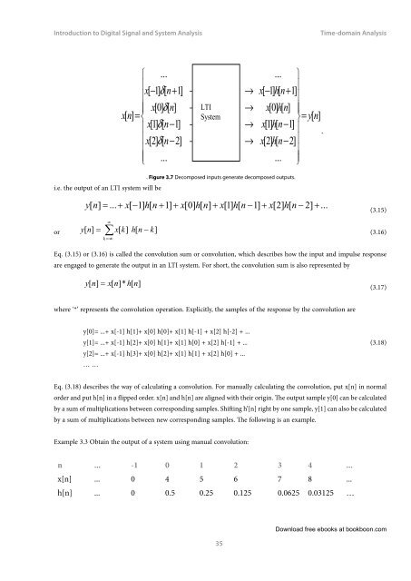
. Figure 3.7 Decomposed inputs generate decomposed outputs.<br />
i.e. the output of an LTI system will be<br />
y[ n]<br />
= ... + x[<br />
−1]<br />
h[<br />
n + 1] + x[0]<br />
h[<br />
n]<br />
+ x[1]<br />
h[<br />
n −1]<br />
+ x[2]<br />
h[<br />
n − 2] + ...<br />
(3.15)<br />
or<br />
∑ ∞<br />
k = −∞<br />
y [ n]<br />
= x[<br />
k]<br />
h[<br />
n − k]<br />
(3.16)<br />
Eq. (3.15) or (3.16) is called the convolution sum or convolution, which describes how the input <strong>and</strong> impulse response<br />
are engaged <strong>to</strong> generate the output in an LTI system. For short, the convolution sum is also represented by<br />
y [ n]<br />
= x[<br />
n]*<br />
h[<br />
n]<br />
(3.17)<br />
where ‘*’ represents the convolution operation. Explicitly, the samples of the response by the convolution are<br />
y[0]= ...+ x[-1] h[1]+ x[0] h[0]+ x[1] h[-1] + x[2] h[-2] + ...<br />
y[1]= ...+ x[-1] h[2]+ x[0] h[1]+ x[1] h[0] + x[2] h[-1] + ... (3.18)<br />
y[2]= ...+ x[-1] h[3]+ x[0] h[2]+ x[1] h[1] + x[2] h[0] + ...<br />
… …<br />
Eq. (3.18) describes the way of calculating a convolution. For manually calculating the convolution, put x[n] in normal<br />
order <strong>and</strong> put h[n] in a flipped order. x[n] <strong>and</strong> h[n] are aligned with their origin. The output sample y[0] can be calculated<br />
by a sum of multiplications between corresponding samples. Shifting h’[n] right by one sample, y[1] can also be calculated<br />
by a sum of multiplications between new corresponding samples. The following is an example.<br />
Example 3.3 Obtain the output of a system using manual convolution:<br />
n ... -1 0 1 2 3 4 ...<br />
x[n] ... 0 4 5 6 7 8 ...<br />
h[n] ... 0 0.5 0.25 0.125 0.0625 0.03125 …<br />
35<br />
Download free ebooks at bookboon.com