Introduction to Digital Signal and System Analysis - Tutorsindia

Introduction to Digital Signal and System Analysis
Z Domain Analysis
z-plane
1
0.8
0.6
0.4
0.2
0
-0.2
-0.4
-0.6
-0.8
-1
-1 -0.5 0 0.5 1
(b)
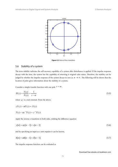
Figure 5.5 Zeros of the z transform
5.6 Stability of a system
The term stability indicates the self-recovery capability of a system after disturbance is applied. If the impulse response
decays with the time, the system has the capability of returning it original calm status. Therefore, the stability can be
judged by whether the impulse response of the system decays to zero as n → ∞ . The following will be shown that the
location of poles gives information about the stability of a system.
Consider a simple transfer function with one pole
z = α :
Y ( z)
1
H ( z)
= = (5.5)
X ( z)
z −α
where α is a real constant. From the above,
zY ( z)
− α Y ( z)
= X ( z)
Y ( z)
−αz
−1
Y ( z)
= z
−1
X ( z)
Apply the inverse z-transform to both sides, yielding the difference equation
y[ n]
= αy[
n −1]
+ x[
n −1]
(5.6)
and by specifying an input as a unit impulse it can be known,
h[ n]
= αh[
n −1]
+ d [ n −1]
(5.7)
The impulse response function can be evaluated as
71
Download free ebooks at bookboon.com