Introduction to Digital Signal and System Analysis - Tutorsindia

Introduction to Digital Signal and System Analysis
Discrete Fourier Transform
6 Discrete Fourier Transform
6.1 Definition of discrete Fourier transform
For a digital signal x [n]
, the discrete Fourier transform (DFT) is defined as
N
= − 1
2πkn
X [ k]
x[
n]exp
− j
n= 0 N (6.1)
where the DFT X [k]
is a discrete periodic function of period N. Therefore one period of distinct values are only taken
at k = 0,1,2,...,
N −1
.
Note that the DFT Eq.(6.1) only has defined the transform over 0 ≤ n ≤ N −1
, otherwise not known or not cared. This
is different from Fourier series in which the signal is strictly periodic or the discrete version of Fourier transform in which
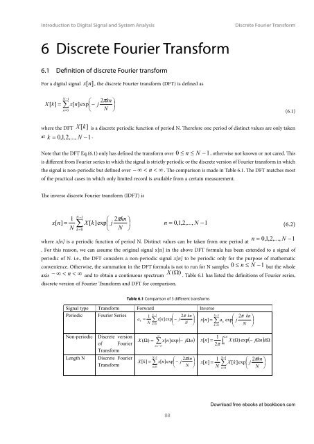
the signal is non-periodic but defined over − ∞ < n < ∞ . The comparison is made in Table 6.1. The DFT matches most
of the practical cases in which only limited record is available from a certain measurement.
The inverse discrete Fourier transform (IDFT) is
N
= − 1
1
2πkn
x[
n]
X [ k]exp
j
N k = 0 N
n = 0,1,2,...,
N −1
(6.2)
where x[n] is a periodic function of period N. Distinct values can be taken from one period at
n = 0,1,2,...,
N −1
. For this reason, we can assume the original signal x[n] in the above DFT formula has been extended to a signal of
periodic of N. i.e., the DFT considers a non-periodic signal x[n] to be periodic only for the purpose of mathematic
convenience. Otherwise, the summation in the DFT formula is not to run for N samples 0 ≤ n ≤ N −1
but the whole
axis − ∞ < n < ∞ and to obtain a continuous spectrum
X (W)
. Table 6.1 has listed the definitions of Fourier series,
discrete version of Fourier Transform and DFT for comparison.
Table 6.1 Comparison of 3 different transforms
Signal type Transform Forward Inverse
Periodic Fourier Series
− 1
1 N 2π
kn
ak
= x[
n]exp
− j
x[
n]
=
N n=
0 N
N
− 1
ak
k = 0
2π
kn
exp
j
N
Non-periodic
Length N
Discrete version
of Fourier
Transform
Discrete Fourier
Transform
X
2π
( Ω)
= x[
n]
exp( − jΩn)
x[
n]
= X ( Ω) exp( − jΩn) dΩ
∞
n=
−∞
N
= − 1
2πkn
X[
k]
x[
n]exp
− j
n= 0 N
x[
n]
1
2π
0
N
= − 1
1
2πkn
X [ k]exp
j
N n= 0 N
88
Download free ebooks at bookboon.com