Introduction to Digital Signal and System Analysis - Tutorsindia

Introduction to Digital Signal and System Analysis
Z Domain Analysis
d)
e)
0.5z
X ( z)
=
2
z − z + 0.5
z − 0.5
X ( z)
=
z(
z − 0.8)( z −1)
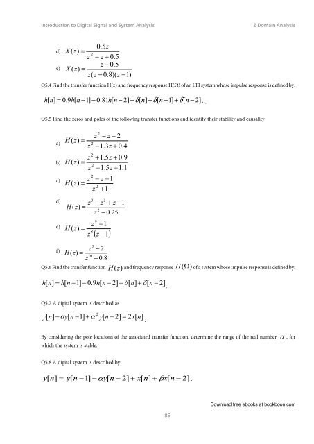
Q5.4 Find the transfer function H(z) and frequency response H(W) of an LTI system whose impulse response is defined by:
h[ n]
= 0.9h[
n −1]
− 0.81h[
n − 2] + δ [ n]
−δ[
n −1]
+ δ[
n − 2] . .
Q5.5 Find the zeros and poles of the following transfer functions and identify their stability and causality:
a)
b)
c)
d)
e)
H ( z)
=
2
z
2
z
H ( z)
=
2
z
H
2
z − z − 2
−1.3z
+ 0.4
+ 1.5z
+ 0.9
−1.5z
+ 1.1
2
z − z + 1
z)
= z + 1
(
2
3 2
z − z + z −1
H ( z)
=
2
z − 0.25
z
H ( z)
=
8
z
9
−1
( z −1)
5
f) z − 2
H ( z)
= z
10
− 0.8
Q5.6 Find the transfer function H (z)
and frequency response H (W)
h[ n]
= h[
n −1]
− 0.9h[
n − 2] + [ n]
+ d[
n − 2]
d
.
of a system whose impulse response is defined by:
Q5.7 A digital system is described as
2
y [ n]
− y[
n −1]
+ α y[
n − 2] = 2x[
n]
α
.
By considering the pole locations of the associated transfer function, determine the range of the real number, α , for
which the system is stable.
Q5.8 A digital system is described by:
y[ n]
= y[
n −1]
−α y[
n − 2] + x[
n]
+ βx[
n − 2] .
85
Download free ebooks at bookboon.com