- Page 1 and 2:
Stochastic Programming Second Editi
- Page 3 and 4:
Contents Preface . . . . . . . . .
- Page 5 and 6:
CONTENTS v 3.6 Simple Recourse . .
- Page 7 and 8:
Preface Over the last few years, bo
- Page 9 and 10:
PREFACE ix more explicitly with the
- Page 11 and 12:
1 Basic Concepts 1.1 Motivation By
- Page 13 and 14:
BASIC CONCEPTS 3 solutions. These a
- Page 15 and 16:
BASIC CONCEPTS 5 will be lost. In s
- Page 17 and 18:
BASIC CONCEPTS 7 1.2 Preliminaries
- Page 19 and 20:
BASIC CONCEPTS 9 with center ˆx an
- Page 21 and 22:
BASIC CONCEPTS 11 Figure 2 Determin
- Page 23 and 24:
BASIC CONCEPTS 13 (except for U). S
- Page 25 and 26:
BASIC CONCEPTS 15 may be wait-and-s
- Page 27 and 28:
BASIC CONCEPTS 17 dual decompositio
- Page 29 and 30:
BASIC CONCEPTS 19 and an empirical
- Page 31 and 32:
BASIC CONCEPTS 21 1.4 Stochastic Pr
- Page 33 and 34:
BASIC CONCEPTS 23 Figure 8 Measure
- Page 35 and 36:
BASIC CONCEPTS 25 These properties
- Page 37 and 38:
BASIC CONCEPTS 27 Figure 10 Classif
- Page 39 and 40:
BASIC CONCEPTS 29 Figure 12 Integra
- Page 41 and 42:
BASIC CONCEPTS 31 µ(A) =0alsoP (A)
- Page 43 and 44:
BASIC CONCEPTS 33 Hence, taking int
- Page 45 and 46:
BASIC CONCEPTS 35 Consequently, for
- Page 47 and 48:
BASIC CONCEPTS 37 Proof For ˆx, ¯
- Page 49 and 50:
BASIC CONCEPTS 39 Figure 13 Linear
- Page 51 and 52:
BASIC CONCEPTS 41 Figure 15 Differe
- Page 53 and 54:
BASIC CONCEPTS 43 However—for fin
- Page 55 and 56:
BASIC CONCEPTS 45 Figure 17 Induced
- Page 57 and 58:
BASIC CONCEPTS 47 Hence the feasibl
- Page 59 and 60:
BASIC CONCEPTS 49 Figure 19 λ = 1
- Page 61 and 62:
BASIC CONCEPTS 51 and hence P (λS
- Page 63 and 64:
BASIC CONCEPTS 53 The sequence of s
- Page 65 and 66:
BASIC CONCEPTS 55 is satisfied. Giv
- Page 67 and 68:
BASIC CONCEPTS 57 Now either z is a
- Page 69 and 70:
BASIC CONCEPTS 59 Figure 22 Polyhed
- Page 71 and 72:
BASIC CONCEPTS 61 Figure 23 Polyhed
- Page 73 and 74:
BASIC CONCEPTS 63 Figure 25 LP: unb
- Page 75 and 76:
BASIC CONCEPTS 65 this case, the re
- Page 77 and 78:
BASIC CONCEPTS 67 Step 3 Exchange t
- Page 79 and 80:
BASIC CONCEPTS 69 bases for any lin
- Page 81 and 82:
BASIC CONCEPTS 71 ✷ Example 1.6 C
- Page 83 and 84:
BASIC CONCEPTS 73 which, observing
- Page 85 and 86:
BASIC CONCEPTS 75 is equal to the p
- Page 87 and 88:
BASIC CONCEPTS 77 solve the program
- Page 89 and 90:
BASIC CONCEPTS 79 {v | Wv =0,q T v0
- Page 91 and 92:
BASIC CONCEPTS 81 The feasible set
- Page 93 and 94:
BASIC CONCEPTS 83 1.8.1 The Kuhn-Tu
- Page 95 and 96:
BASIC CONCEPTS 85 Figure 28 Kuhn-Tu
- Page 97 and 98:
BASIC CONCEPTS 87 Figure 29 The Sla
- Page 99 and 100:
BASIC CONCEPTS 89 and observing tha
- Page 101 and 102:
BASIC CONCEPTS 91 where the bounded
- Page 103 and 104:
BASIC CONCEPTS 93 λŷ +(1− λ)ˆ
- Page 105 and 106:
BASIC CONCEPTS 95 “reasonable”
- Page 107 and 108:
BASIC CONCEPTS 97 1.8.2.3 Penalty m
- Page 109 and 110:
BASIC CONCEPTS 99 To simplify the d
- Page 111 and 112:
BASIC CONCEPTS 101 Now let us come
- Page 113 and 114:
BASIC CONCEPTS 103 Wait-and-see pro
- Page 115 and 116:
BASIC CONCEPTS 105 y ≤ e −x } f
- Page 117 and 118:
BASIC CONCEPTS 107 Optimization: No
- Page 119 and 120:
2 Dynamic Systems 2.1 The Bellman P
- Page 121 and 122:
112 STOCHASTIC PROGRAMMING purpose
- Page 123 and 124:
114 STOCHASTIC PROGRAMMING In this
- Page 125 and 126:
116 STOCHASTIC PROGRAMMING Proof Th
- Page 127 and 128:
118 STOCHASTIC PROGRAMMING A 10% fe
- Page 129 and 130:
120 STOCHASTIC PROGRAMMING Stage 0
- Page 131 and 132:
122 STOCHASTIC PROGRAMMING Stage 0
- Page 133 and 134:
124 STOCHASTIC PROGRAMMING Table 1
- Page 135 and 136:
126 STOCHASTIC PROGRAMMING Stage 0
- Page 137 and 138:
128 STOCHASTIC PROGRAMMING situatio
- Page 139 and 140:
130 STOCHASTIC PROGRAMMING 2.5 Stoc
- Page 141 and 142:
132 STOCHASTIC PROGRAMMING Using th
- Page 143 and 144:
134 STOCHASTIC PROGRAMMING 2.6 Scen
- Page 145 and 146:
136 STOCHASTIC PROGRAMMING Today Fi
- Page 147 and 148:
138 STOCHASTIC PROGRAMMING procedur
- Page 149 and 150:
140 STOCHASTIC PROGRAMMING the natu
- Page 151 and 152:
142 STOCHASTIC PROGRAMMING book, be
- Page 153 and 154:
144 STOCHASTIC PROGRAMMING • A tw
- Page 155 and 156:
146 STOCHASTIC PROGRAMMING Figu
- Page 157 and 158:
148 STOCHASTIC PROGRAMMING 2.8.1 A
- Page 159 and 160:
150 STOCHASTIC PROGRAMMING 2.8.2 Fu
- Page 161 and 162:
152 STOCHASTIC PROGRAMMING 2.9.2 De
- Page 163 and 164:
154 STOCHASTIC PROGRAMMING between
- Page 165 and 166:
156 STOCHASTIC PROGRAMMING an exerc
- Page 167 and 168:
158 STOCHASTIC PROGRAMMING
- Page 169 and 170:
160 STOCHASTIC PROGRAMMING
- Page 171 and 172:
162 STOCHASTIC PROGRAMMING Hξ pos
- Page 173 and 174:
164 STOCHASTIC PROGRAMMING pos W po
- Page 175 and 176:
166 STOCHASTIC PROGRAMMING Figure
- Page 177 and 178:
168 STOCHASTIC PROGRAMMING procedur
- Page 179 and 180:
170 STOCHASTIC PROGRAMMING procedur
- Page 181 and 182:
172 STOCHASTIC PROGRAMMING θ Q(x)
- Page 183 and 184:
174 STOCHASTIC PROGRAMMING • If t
- Page 185 and 186:
176 STOCHASTIC PROGRAMMING Figure 1
- Page 187 and 188:
178 STOCHASTIC PROGRAMMING is diffi
- Page 189 and 190:
180 STOCHASTIC PROGRAMMING lower-bo
- Page 191 and 192:
182 STOCHASTIC PROGRAMMING Edmundso
- Page 193 and 194:
184 STOCHASTIC PROGRAMMING Edmundso
- Page 195 and 196:
186 STOCHASTIC PROGRAMMING The goal
- Page 197 and 198:
188 STOCHASTIC PROGRAMMING which eq
- Page 199 and 200:
190 STOCHASTIC PROGRAMMING random v
- Page 201 and 202:
192 STOCHASTIC PROGRAMMING increase
- Page 203 and 204:
194 STOCHASTIC PROGRAMMING φ β α
- Page 205 and 206:
196 STOCHASTIC PROGRAMMING change i
- Page 207 and 208:
198 STOCHASTIC PROGRAMMING Figure 2
- Page 209 and 210:
200 STOCHASTIC PROGRAMMING The mini
- Page 211 and 212:
202 STOCHASTIC PROGRAMMING
- Page 213 and 214:
204 STOCHASTIC PROGRAMMING procedur
- Page 215 and 216:
206 STOCHASTIC PROGRAMMING Hence, w
- Page 217 and 218:
208 STOCHASTIC PROGRAMMING Figure 2
- Page 219 and 220:
210 STOCHASTIC PROGRAMMING since th
- Page 221 and 222:
212 STOCHASTIC PROGRAMMING or later
- Page 223 and 224:
214 STOCHASTIC PROGRAMMING problem
- Page 225 and 226:
216 STOCHASTIC PROGRAMMING procedur
- Page 227 and 228:
218 STOCHASTIC PROGRAMMING where
- Page 229 and 230:
220 STOCHASTIC PROGRAMMING Remember
- Page 231 and 232:
222 STOCHASTIC PROGRAMMING φ ( ) F
- Page 233 and 234:
224 STOCHASTIC PROGRAMMING
- Page 235 and 236:
226 STOCHASTIC PROGRAMMING By assum
- Page 237 and 238:
228 STOCHASTIC PROGRAMMING Figure 3
- Page 239 and 240:
230 STOCHASTIC PROGRAMMING work, wh
- Page 241 and 242:
232 STOCHASTIC PROGRAMMING problem.
- Page 243 and 244:
234 STOCHASTIC PROGRAMMING Madansky
- Page 245 and 246: 236 STOCHASTIC PROGRAMMING 5. Show
- Page 247 and 248: 238 STOCHASTIC PROGRAMMING [16] Dup
- Page 249 and 250: 240 STOCHASTIC PROGRAMMING J.-B. (e
- Page 251 and 252: 242 STOCHASTIC PROGRAMMING
- Page 253 and 254: 244 STOCHASTIC PROGRAMMING Proposit
- Page 255 and 256: 246 STOCHASTIC PROGRAMMING (f T ,g
- Page 257 and 258: 248 STOCHASTIC PROGRAMMING covarian
- Page 259 and 260: 250 STOCHASTIC PROGRAMMING With the
- Page 261 and 262: 252 STOCHASTIC PROGRAMMING It is st
- Page 263 and 264: 254 STOCHASTIC PROGRAMMING Hence we
- Page 265 and 266: 256 STOCHASTIC PROGRAMMING Taking t
- Page 267 and 268: 258 STOCHASTIC PROGRAMMING reader m
- Page 269 and 270: 260 STOCHASTIC PROGRAMMING
- Page 271 and 272: 262 STOCHASTIC PROGRAMMING procedur
- Page 273 and 274: 264 STOCHASTIC PROGRAMMING that is,
- Page 275 and 276: 266 STOCHASTIC PROGRAMMING pos W po
- Page 277 and 278: 268 STOCHASTIC PROGRAMMING procedur
- Page 279 and 280: 270 STOCHASTIC PROGRAMMING Figure 7
- Page 281 and 282: 272 STOCHASTIC PROGRAMMING min{2x r
- Page 283 and 284: 274 STOCHASTIC PROGRAMMING directio
- Page 285 and 286: 276 STOCHASTIC PROGRAMMING [5] Gree
- Page 287 and 288: 278 STOCHASTIC PROGRAMMING outlined
- Page 289 and 290: 280 STOCHASTIC PROGRAMMING since we
- Page 291 and 292: 282 STOCHASTIC PROGRAMMING 2 1 a b
- Page 293 and 294: 284 STOCHASTIC PROGRAMMING procedur
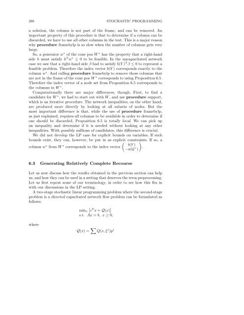
- Page 295: 286 STOCHASTIC PROGRAMMING 6.2.1 Th
- Page 299 and 300: 290 STOCHASTIC PROGRAMMING Since th
- Page 301 and 302: 292 STOCHASTIC PROGRAMMING It is no
- Page 303 and 304: 294 STOCHASTIC PROGRAMMING [-1,1] [
- Page 305 and 306: 296 STOCHASTIC PROGRAMMING for some
- Page 307 and 308: 298 STOCHASTIC PROGRAMMING +/- 1 1
- Page 309 and 310: 300 STOCHASTIC PROGRAMMING 1 (-1,0)
- Page 311 and 312: 302 STOCHASTIC PROGRAMMING with a g
- Page 313 and 314: 304 STOCHASTIC PROGRAMMING First, i
- Page 315 and 316: 306 STOCHASTIC PROGRAMMING Table 1
- Page 317 and 318: 308 STOCHASTIC PROGRAMMING Figure 2
- Page 319 and 320: 310 STOCHASTIC PROGRAMMING Universi
- Page 321 and 322: 312 STOCHASTIC PROGRAMMING
- Page 323 and 324: 314 STOCHASTIC PROGRAMMING duality
- Page 325 and 326: 316 STOCHASTIC PROGRAMMING best-so-


