X-ray Study of Low-mass Young Stellar Objects in the ρ Ophiuchi ...

More documents

Recommendations

Info

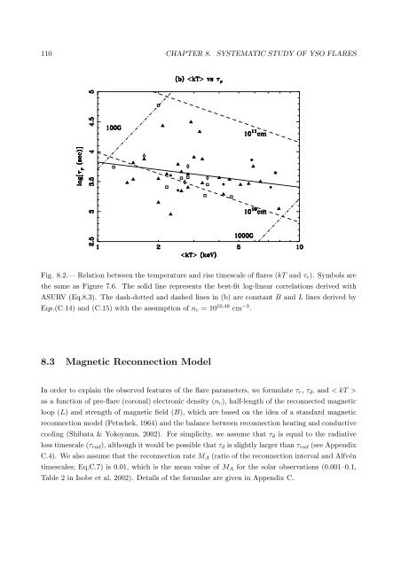
110 CHAPTER 8. SYSTEMATIC STUDY OF YSO FLARESFig. 8.2.— Relation between the temperature and rise timescale of flares (kT and τ r ). Symbols arethe same as Figure 7.6. The solid line represents the best-fit log-linear correlations derived withASURV (Eq.8.3). The dash-dotted and dashed lines in (b) are constant B and L lines derived byEqs.(C.14) and (C.15) with the assumption of n c = 10 10.48 cm −3 .8.3 Magnetic Reconnection ModelIn order to explain the observed features of the flare parameters, we formulate τ r , τ d , and < kT >as a function of pre-flare (coronal) electronic density (n c ), half-length of the reconnected magneticloop (L) and strength of magnetic field (B), which are based on the idea of a standard magneticreconnection model (Petschek, 1964) and the balance between reconnection heating and conductivecooling (Shibata & Yokoyama, 2002). For simplicity, we assume that τ d is equal to the radiativeloss timescale (τ rad ), although it would be possible that τ d is slightly larger than τ rad (see AppendixC.4). We also assume that the reconnection rate M A (ratio of the reconnection interval and Alfvéntimescales; Eq.C.7) is 0.01, which is the mean value of M A for the solar observations (0.001–0.1,Table 2 in Isobe et al. 2002). Details of the formulae are given in Appendix C.
8.3. MAGNETIC RECONNECTION MODEL 1118.3.1 τ r vs τ d – Implication of the pre-flare densityFrom Eq.(C.12), the reconnection model predicts the positive correlation between τ r and τ d asτ d = Aτr1/2 . The slope of 1/2 shows good agreement with the observed value of 0.4±0.1 (Eq.8.2),hence supports our assumption that the decay phase is dominant by radiative cooling. FromEq.(C.12), we re-estimate log(A) with the fixed slope of 1/2 to be 2.06±0.04 (the dashed line inFigure 8.1). We also calculate log(A) separately for each class, then obtain 2.1±0.1, 2.0±0.1, and2.0±0.1 for class I, II, and III+III c , respectively. We see no significant difference between theclasses, hence A is assumed to be the same for all sources. Since A is a function of n c (Eq.C.13),we can determine n c to ben c = 10 10.48±0.09 ( M A0.01 ) [cm−3 ]. (8.4)Considering the possible range of M A (0.001–0.1), this favors higher pre-flare density for YSOs(10 9 –10 12 cm −3 ) than that for the sun (∼10 9 cm −3 ). In fact, Kastner et al. (2002) derived theplasma density of a CTTS (TW Hydrae) using the ratio of Ne IX and O VII triplets and foundextremely high density of ∼10 13 cm −3 even in their quiescent phase. Hence larger n c value forYSOs than that for the sun would be common feature.8.3.2 < kT > vs τ r – Loop length and magnetic field strengthThe predicted correlations between < kT > and τ r are shown in Eqs. (C.14) and (C.15). Positive(τ r ∝< kT > 7/2 ) and negative (τ r ∝< kT > −7/6 ) correlations are expected for the constant Band L values, respectively. The dash-dotted and dashed lines in Figure 8.2 show the constant Band L lines, in which we uniformly assume n c = 10 10.48 cm −3 (Eq.8.4). Our observed negativecorrelation therefore predicts that flares with higher temperature is mainly due to larger magneticfield. However, the observed slope of −0.4±0.3 is significantly flatter than −7/6 (Eq. C.15), hencethe effect of L would not be negligible. We estimate the mean B and L for each class (Table 8.2)using the mean values of < kT > and τ r (Figures 7.4b and 7.5a), which is summarized in Table8.2. Younger sources tend to show larger B values; the mean values of B are ∼500, 300, and 200 Gfor class I, II, and III+III c sources, respectively. This is consistent with the observed result ofhigher plasma temperature for younger sources. Also, the estimated values of L (10 10 –10 11 cm)suggest that L is nearly the same among these classes, comparable to the typical radius of YSOs.These results indicate that the flare loops for all classes are localized at the stellar surface, whichis in sharp contrast with the idea of the flares for class I sources triggered by the larger flare loopsconnecting the star and the disk (Montmerle et al., 2000).It is conceivable that the class III flares with unusually long timescales (A-2, A-63, and BF-96)mainly affect the systematically lower B for class III sources. Since it is possible that two or more
Page 3:
Contents1 Introduction 12 Review of
Page 9 and 10:
List of Figures2.1 The H-R diagram
Page 11 and 12:
LIST OF FIGURESix6.17 Light curves
Page 13 and 14:
List of Tables3.1 Multiwavelength s
Page 15 and 16:
Chapter 1IntroductionStar formation
Page 17 and 18:
Chapter 2Review of Low-mass Young S
Page 19 and 20:
2.1. EVOLUTION OF LOW-MASS STARS 5w
Page 21 and 22:
2.2. MOLECULAR CLOUDS 72.2 Molecula
Page 23 and 24:
2.3. X-RAY OBSERVATIONS OF LOW-MASS
Page 25 and 26:
Page 27:
Page 30 and 31:
16 CHAPTER 3. REVIEW OF THE ρ OPHI
Page 32 and 33:
Page 34 and 35:
Page 36 and 37:
22 CHAPTER 4. INSTRUMENTATIONrespec
Page 38 and 39:
24 CHAPTER 4. INSTRUMENTATIONangle
Page 40 and 41:
26 CHAPTER 4. INSTRUMENTATIONThe AC
Page 42 and 43:
¨28 CHAPTER 4. INSTRUMENTATIONspli
Page 44 and 45:
30 CHAPTER 4. INSTRUMENTATIONTable
Page 46 and 47:
32 CHAPTER 5. CHANDRA OBSERVATIONS
Page 48 and 49:
Page 50 and 51:
Page 52 and 53:
Page 54 and 55:
Page 56 and 57:
Page 58 and 59:
Page 60 and 61:
Page 62 and 63:
Page 64 and 65:
Page 66 and 67:
Page 68 and 69:
Page 70 and 71:
Page 72 and 73:
58 CHAPTER 6. INDIVIDUAL SOURCEShig
Page 74 and 75: 60 CHAPTER 6. INDIVIDUAL SOURCESres
Page 76 and 77: 62 CHAPTER 6. INDIVIDUAL SOURCES6.2
Page 78 and 79: 64 CHAPTER 6. INDIVIDUAL SOURCESfla
Page 80 and 81: 66 CHAPTER 6. INDIVIDUAL SOURCESTab
Page 82 and 83: 68 CHAPTER 6. INDIVIDUAL SOURCESUsi
Page 84 and 85: 70 CHAPTER 6. INDIVIDUAL SOURCESlos
Page 88 and 89: 74 CHAPTER 6. INDIVIDUAL SOURCESdes
Page 90 and 91: 76 CHAPTER 6. INDIVIDUAL SOURCESocc
Page 100 and 101: 86 CHAPTER 6. INDIVIDUAL SOURCEStha
Page 102 and 103: 88 CHAPTER 6. INDIVIDUAL SOURCES1ke
Page 104 and 105: 90 CHAPTER 6. INDIVIDUAL SOURCESThe
Page 106 and 107: 92 CHAPTER 6. INDIVIDUAL SOURCESFig
Page 108 and 109: 94 CHAPTER 6. INDIVIDUAL SOURCESPra
Page 110 and 111: 96 CHAPTER 7. OVERALL FEATURE OF X-
Page 112 and 113: 98 CHAPTER 7. OVERALL FEATURE OF X-
Page 114 and 115: 100 CHAPTER 7. OVERALL FEATURE OF X
Page 121 and 122: Chapter 8Systematic Study of YSO Fl
Page 123: 8.2. CORRELATION BETWEEN THE FLARE
Page 127 and 128: 8.5. EFFECT OF THE QUIESCENT X-RAYS
Page 129 and 130: 8.6. EVOLUTION OF YSOS AND THEIR FL
Page 131 and 132: Chapter 9ConclusionWe summarize the
Page 133 and 134: Appendix AFlare Light CurvesFig. A.
Page 135 and 136: Fig.A.2 (Continued)121
Page 137: Fig. A.4.— Same as Figure A.1, bu
Page 140 and 141: 126 APPENDIX B. PHYSICAL PARAMETERS
Page 142 and 143: 128 APPENDIX B. PHYSICAL PARAMETERS
Page 145 and 146: Appendix CModeling of the FlareIn t
Page 147 and 148: C.2. PREDICTED CORRELATIONS BETWEEN
Page 149 and 150: BibliographyAgeorges, N., Eckart, A
Page 151 and 152: BIBLIOGRAPHY 137Feigelson, E. D., &
Page 153 and 154: BIBLIOGRAPHY 139Johnstone, D., Wils
Page 155 and 156: BIBLIOGRAPHY 141Rutledge, R. E., Ba
Page 157: BIBLIOGRAPHY 143Yokoyama, T. & Shib
show all

X-ray Study of Low-mass Young Stellar Objects in the ρ Ophiuchi ...

Create successful ePaper yourself

Delete template?

Save as template?