X-ray Study of Low-mass Young Stellar Objects in the ρ Ophiuchi ...

More documents

Recommendations

Info

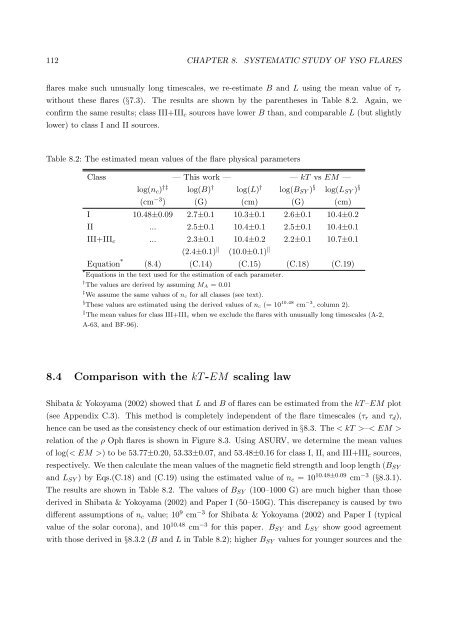
112 CHAPTER 8. SYSTEMATIC STUDY OF YSO FLARESflares make such unusually long timescales, we re-estimate B and L using the mean value of τ rwithout these flares (§7.3). The results are shown by the parentheses in Table 8.2. Again, weconfirm the same results; class III+III c sources have lower B than, and comparable L (but slightlylower) to class I and II sources.Table 8.2: The estimated mean values of the flare physical parametersClass — This work — — kT vs EM —log(n c ) †‡ log(B) † log(L) † log(B SY ) § log(L SY ) §(cm −3 ) (G) (cm) (G) (cm)I 10.48±0.09 2.7±0.1 10.3±0.1 2.6±0.1 10.4±0.2II ... 2.5±0.1 10.4±0.1 2.5±0.1 10.4±0.1III+III c ... 2.3±0.1 10.4±0.2 2.2±0.1 10.7±0.1(2.4±0.1) ‖ (10.0±0.1) ‖Equation * (8.4) (C.14) (C.15) (C.18) (C.19)* Equations in the text used for the estimation of each parameter.† The values are derived by assuming M A = 0.01‡ We assume the same values of n c for all classes (see text).§ These values are estimated using the derived values of n c (= 10 10.48 cm −3 , column 2).‖ The mean values for class III+III c when we exclude the flares with unusually long timescales (A-2,A-63, and BF-96).8.4 Comparison with the kT -EM scaling lawShibata & Yokoyama (2002) showed that L and B of flares can be estimated from the kT –EM plot(see Appendix C.3). This method is completely independent of the flare timescales (τ r and τ d ),hence can be used as the consistency check of our estimation derived in §8.3. The < kT >–relation of the ρ Oph flares is shown in Figure 8.3. Using ASURV, we determine the mean valuesof log() to be 53.77±0.20, 53.33±0.07, and 53.48±0.16 for class I, II, and III+III c sources,respectively. We then calculate the mean values of the magnetic field strength and loop length (B SYand L SY ) by Eqs.(C.18) and (C.19) using the estimated value of n c = 10 10.48±0.09 cm −3 (§8.3.1).The results are shown in Table 8.2. The values of B SY (100–1000 G) are much higher than thosederived in Shibata & Yokoyama (2002) and Paper I (50–150G). This discrepancy is caused by twodifferent assumptions of n c value; 10 9 cm −3 for Shibata & Yokoyama (2002) and Paper I (typicalvalue of the solar corona), and 10 10.48 cm −3 for this paper. B SY and L SY show good agreementwith those derived in §8.3.2 (B and L in Table 8.2); higher B SY values for younger sources and the
8.5. EFFECT OF THE QUIESCENT X-RAYS ON THE FLARE ANALYSIS 113same order of L SY comparable to the typical stellar radius. Therefore our estimation of n c , L, andB using the τ r –τ d and < kT >–τ r relations is cross-checked.The same conclusion of §8.3 and this section also indicates the propriety of our assumption ofM A = 0.01. If we assume the smaller (or larger) value of M A , n c (Eq.8.4) becomes smaller (larger),which causes smaller (larger) estimations of B SY (Eq.C.18) and makes larger discrepancy betweenB and B SY (Table 8.2).Fig. 8.3.— Plot of < kT > and in theflare phases. Symbols are the same as Figure 7.6.The dashed-dotted and dashed lines are constantB and L lines derived by Eqs.(C.18) and (C.19)with the assumption of n c = 10 10.48 cm −3 .8.5 Effect of the Quiescent X-rays on the Flare AnalysisIt is conceivable that the quiescent X-rays put significant influence on the results of our flareanalysis. Hence, in this subsection, we make and fit the flare spectra by subtracting the quiescentspectra as a background level and compare the results with those in the previous section. For thespectral fittings, the absorption column (N H ) is fixed to be the best-fit value in Table 5.2.Figure 8.4 shows the histogram of the newly estimated < kT > in the flare phases. Since thestatistics are highly limited due to the higher background level than that for the previous analysis,many faint flares can not constrain the 90 % confidence limit of < kT >. Hence, we only use thedata whose errors are well determined. Although the mean values of < kT > are systematicallyhigher and lower than the previous results, overall properties are the same; higher < kT > for classI and II sources than class III+III c . Using ASURV, the significance level of higher < kT > for classI and II sources is estimated to be 92 %. This value is a bit smaller than the previous analysis(Table 7.2), which would be simply due to the limited samples for this analysis.The plot of < kT > and τ r is shown in Figure 8.5. Similar to Figure 8.4, we only use thedata whose 90 % confidence limit is well determined. The mean values of L are ∼2.6, 2.7, and3.1 ×10 10 cm, while those of B are ∼600, 300, and 200 G for class I, II and III+III c , respectively.
Page 3:
Contents1 Introduction 12 Review of
Page 9 and 10:
List of Figures2.1 The H-R diagram
Page 11 and 12:
LIST OF FIGURESix6.17 Light curves
Page 13 and 14:
List of Tables3.1 Multiwavelength s
Page 15 and 16:
Chapter 1IntroductionStar formation
Page 17 and 18:
Chapter 2Review of Low-mass Young S
Page 19 and 20:
2.1. EVOLUTION OF LOW-MASS STARS 5w
Page 21 and 22:
2.2. MOLECULAR CLOUDS 72.2 Molecula
Page 23 and 24:
2.3. X-RAY OBSERVATIONS OF LOW-MASS
Page 25 and 26:
Page 27:
Page 30 and 31:
16 CHAPTER 3. REVIEW OF THE ρ OPHI
Page 32 and 33:
Page 34 and 35:
Page 36 and 37:
22 CHAPTER 4. INSTRUMENTATIONrespec
Page 38 and 39:
24 CHAPTER 4. INSTRUMENTATIONangle
Page 40 and 41:
26 CHAPTER 4. INSTRUMENTATIONThe AC
Page 42 and 43:
¨28 CHAPTER 4. INSTRUMENTATIONspli
Page 44 and 45:
30 CHAPTER 4. INSTRUMENTATIONTable
Page 46 and 47:
32 CHAPTER 5. CHANDRA OBSERVATIONS
Page 48 and 49:
Page 50 and 51:
Page 52 and 53:
Page 54 and 55:
Page 56 and 57:
Page 58 and 59:
Page 60 and 61:
Page 62 and 63:
Page 64 and 65:
Page 66 and 67:
Page 68 and 69:
Page 70 and 71:
Page 72 and 73:
58 CHAPTER 6. INDIVIDUAL SOURCEShig
Page 74 and 75:
60 CHAPTER 6. INDIVIDUAL SOURCESres
Page 76 and 77: 62 CHAPTER 6. INDIVIDUAL SOURCES6.2
Page 78 and 79: 64 CHAPTER 6. INDIVIDUAL SOURCESfla
Page 80 and 81: 66 CHAPTER 6. INDIVIDUAL SOURCESTab
Page 82 and 83: 68 CHAPTER 6. INDIVIDUAL SOURCESUsi
Page 84 and 85: 70 CHAPTER 6. INDIVIDUAL SOURCESlos
Page 88 and 89: 74 CHAPTER 6. INDIVIDUAL SOURCESdes
Page 90 and 91: 76 CHAPTER 6. INDIVIDUAL SOURCESocc
Page 100 and 101: 86 CHAPTER 6. INDIVIDUAL SOURCEStha
Page 102 and 103: 88 CHAPTER 6. INDIVIDUAL SOURCES1ke
Page 104 and 105: 90 CHAPTER 6. INDIVIDUAL SOURCESThe
Page 106 and 107: 92 CHAPTER 6. INDIVIDUAL SOURCESFig
Page 108 and 109: 94 CHAPTER 6. INDIVIDUAL SOURCESPra
Page 110 and 111: 96 CHAPTER 7. OVERALL FEATURE OF X-
Page 112 and 113: 98 CHAPTER 7. OVERALL FEATURE OF X-
Page 114 and 115: 100 CHAPTER 7. OVERALL FEATURE OF X
Page 121 and 122: Chapter 8Systematic Study of YSO Fl
Page 123 and 124: 8.2. CORRELATION BETWEEN THE FLARE
Page 125: 8.3. MAGNETIC RECONNECTION MODEL 11
Page 129 and 130: 8.6. EVOLUTION OF YSOS AND THEIR FL
Page 131 and 132: Chapter 9ConclusionWe summarize the
Page 133 and 134: Appendix AFlare Light CurvesFig. A.
Page 135 and 136: Fig.A.2 (Continued)121
Page 137: Fig. A.4.— Same as Figure A.1, bu
Page 140 and 141: 126 APPENDIX B. PHYSICAL PARAMETERS
Page 142 and 143: 128 APPENDIX B. PHYSICAL PARAMETERS
Page 145 and 146: Appendix CModeling of the FlareIn t
Page 147 and 148: C.2. PREDICTED CORRELATIONS BETWEEN
Page 149 and 150: BibliographyAgeorges, N., Eckart, A
Page 151 and 152: BIBLIOGRAPHY 137Feigelson, E. D., &
Page 153 and 154: BIBLIOGRAPHY 139Johnstone, D., Wils
Page 155 and 156: BIBLIOGRAPHY 141Rutledge, R. E., Ba
Page 157: BIBLIOGRAPHY 143Yokoyama, T. & Shib
show all

X-ray Study of Low-mass Young Stellar Objects in the ρ Ophiuchi ...

Create successful ePaper yourself

Delete template?

Save as template?