Applications of state space models in finance

114 6 Time-varying market beta risk of pan-European sectors
mean error
3.0
2.5
2.0
1.5
1.0
0.5
(a) Average mean errors
MAE
MSE
0.0
OLS tG MSM MS GRW SV RW MR MMR
rank
8
6
4
2
(b) Average ranks
MAE
MSE
0
OLS tG MSM MS GRW SV RW MR MMR
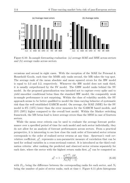
Figure 6.10: In-sample forecasting evaluation: (a) average MAE and MSE across sectors
and (b) average ranks across sectors.
occasions and second in eight cases. With the exception of the MAE for Personal &
Household Goods, each time the MMR only ranks second, the MR takes the top spot.
The average rank of the mean absolute and mean squared errors for the RW model
is equal to 3.3 and 3.2, respectively. Whenever the RW model does not rank third,
it is usually outperformed by the SV model. The GRW model ranks behind the SV
model. As the proposed generalization was intended not to capture every spike and to
yield smoother conditional betas than the standard RW model, the comparably weak
in-sample performance is not surprising. Within the class of volatility models, the SV
approach seems to be better qualified to model the time-varying behavior of systematic
risk than the well established GARCH model. On average, the MAE (MSE) for the SV
model is 6% (13%) lower than the error measures for the GARCH based models, and
25% (59%) higher compared to the overall best model. Within the Markov switching
framework, the MS betas lead to lower average errors than the MSM in case of fourteen
sectors.
While the mean error criteria can be used to evaluate the average forecast performance
over a specified period of time for each model and each sector individually, they
do not allow for an analysis of forecast performances across sectors. From a practical
perspective, it is interesting to see how close the rank order of forecasted sector returns
corresponds to the order of realized sector returns at any time. Spearman’s rank correlation
coefficient, ρS t , represents a non-parametric measure of correlation that can be
used for ordinal variables in a cross-sectional context. It is introduced as the third eval-
uation criteria: after ranking the predicted and observed sector returns separately for
each date, where the sector with the highest return ranks first, ρS t can be computed as
i=1 D2 i,t
Nt(N 2 t − 1)
ρ S t = 1 − 6 � Nt
, (6.43)
with Di,t being the difference between the corresponding ranks for each sector, and Nt
being the number of pairs of sector ranks, each at time t. Figure 6.11 plots histograms