Applications of state space models in finance
Applications of state space models in finance
Applications of state space models in finance
You also want an ePaper? Increase the reach of your titles
YUMPU automatically turns print PDFs into web optimized ePapers that Google loves.
3.6 Model diagnostics 37<br />
3.6.1 Residuals<br />
¢<br />
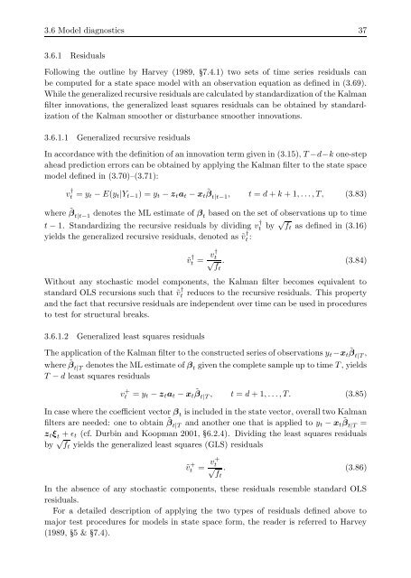
Follow<strong>in</strong>g the outl<strong>in</strong>e by Harvey (1989, 7.4.1) two sets <strong>of</strong> time series residuals can<br />
be computed for a <strong>state</strong> <strong>space</strong> model with an observation equation as def<strong>in</strong>ed <strong>in</strong> (3.69).<br />
While the generalized recursive residuals are calculated by standardization <strong>of</strong> the Kalman<br />
filter <strong>in</strong>novations, the generalized least squares residuals can be obta<strong>in</strong>ed by standardization<br />
<strong>of</strong> the Kalman smoother or disturbance smoother <strong>in</strong>novations.<br />
3.6.1.1 Generalized recursive residuals<br />
In accordance with the def<strong>in</strong>ition <strong>of</strong> an <strong>in</strong>novation term given <strong>in</strong> (3.15), T −d−k one-step<br />
ahead prediction errors can be obta<strong>in</strong>ed by apply<strong>in</strong>g the Kalman filter to the <strong>state</strong> <strong>space</strong><br />
model def<strong>in</strong>ed <strong>in</strong> (3.70)–(3.71):<br />
v †<br />
t = yt − E(yt|Yt−1) = yt − ztat − xt ˜ β t|t−1 , t = d + k + 1, . . . , T, (3.83)<br />
where ˜ βt|t−1 denotes the ML estimate <strong>of</strong> βt based on the set <strong>of</strong> observations up to time<br />
t − 1. Standardiz<strong>in</strong>g the recursive residuals by divid<strong>in</strong>g v †<br />
t by √ ft as def<strong>in</strong>ed <strong>in</strong> (3.16)<br />
yields the generalized recursive residuals, denoted as ˜v †<br />
t :<br />
t = v† t √<br />
ft<br />
˜v †<br />
. (3.84)<br />
Without any stochastic model components, the Kalman filter becomes equivalent to<br />
standard OLS recursions such that ˜v †<br />
t reduces to the recursive residuals. This property<br />
and the fact that recursive residuals are <strong>in</strong>dependent over time can be used <strong>in</strong> procedures<br />
to test for structural breaks.<br />
3.6.1.2 Generalized least squares residuals<br />
The application <strong>of</strong> the Kalman filter to the constructed series <strong>of</strong> observations yt−xt ˜ β t|T ,<br />
where ˜ β t|T denotes the ML estimate <strong>of</strong> β t given the complete sample up to time T , yields<br />
T − d least squares residuals<br />
v + t = yt − ztat − xt ˜ β t|T , t = d + 1, . . . , T. (3.85)<br />
In case where the coefficient vector β t is <strong>in</strong>cluded <strong>in</strong> the <strong>state</strong> vector, overall two Kalman<br />
filters are needed: one to obta<strong>in</strong> ˜ β t|T and another one that is applied to yt − xt ˜ β t|T =<br />
ztξ t + ɛt (cf. Durb<strong>in</strong> and Koopman 2001, ¢ 6.2.4). Divid<strong>in</strong>g the least squares residuals<br />
by √ ft yields the generalized least squares (GLS) residuals<br />
˜v + t = v+ t √ft . (3.86)<br />
In the absence <strong>of</strong> any stochastic components, these residuals resemble standard OLS<br />
residuals.<br />
For a detailed description <strong>of</strong> apply<strong>in</strong>g the two types <strong>of</strong> residuals def<strong>in</strong>ed above to<br />
major test procedures for <strong>models</strong> <strong>in</strong> <strong>state</strong> <strong>space</strong> form, the reader is referred to Harvey<br />
(1989, ¢ 5 & ¢ 7.4).


