Applications of state space models in finance

More documents

Recommendations

Info

116 6 Time-varying market beta risk of pan-European sectors model gives a satisfactory description of historical phenomena does not [. . . ] mean that it will perform as well on the future.” Therefore, the indispensable extension to the model comparisons conducted above is to evaluate the respective out-of-sample forecast performances. In a first step, 100 beta and return forecasts based on 100 samples of 520 weekly observations are estimated for all proposed time-varying techniques. Within this rolling window forecasting procedure, the sample is rolled forward by one week, while the sample size is kept constant at 520. The first sample starts 24 March 1993 and ends 5 March 2003. It is used to calculate the out-of-sample conditional beta forecasts for 12 March 2003 based on the chosen modeling technique. The 100-th beta forecast for 2 February 2005 is then generated based on the last sample starting 15 February 1995 and ending 26 January 2005. The reason why the out-of-sample period is chosen to be limited to one hundred observations is to ensure proper convergence of the conditional volatility models. As will be seen from this analysis, the three Kalman filter based models RW, MMR and GRW prove to be superior in an out-of-sample context. In a second step, an out-of-sample period of ten years based on 520 samples of 150 weekly observations is considered for these three models. As the Kalman filter does not require as many observations as the GARCH or stochastic volatility based models, an analysis based on an extended out-of-sample period is added. An estimation period of 150 weeks is chosen to allow for an out-of-sample period of 10 years for all eighteen sectors, including the three newly formed sectors for which only 683 instead of 897 weekly observations are available. An estimation period of 150 data points is somehow arbitrary and represents a compromise. According to Lo and MacKinlay (1997, ¢ 5.1) the most common choice to estimate the market model is to employ five years of monthly data. The current chapter deals with the forecastability of systematic risk at a more shortterm horizon, which is reflected by the use of weekly data. Therefore, an estimation period roughly corresponding to three years of data is justified: while it contains enough data to generate stable parameter estimates, it is short enough to reflect current market conditions. Remembering that the Kalman filter naturally puts more weight on the most recent observations, the out-of-sample results for the Kalman filter models do not critically depend on the length of the estimation period. The goal of this analysis is to identify the Kalman filter model that generates the best out-of-sample forecasts of the time-varying exposure to systematic risk over the more representative time horizon of ten years. The to be identified overall best approach will be chosen in the next chapter to model and forecast the time-varying relationship between macroeconomics and sector allocation. 6.3.3.1 Step I: Out-of-sample period of 100 weeks to compare all conditional modeling techniques To compare the out-of-sample performances of all conditional betas, the average MAE and MSE measures across sectors and the respective average ranks are shown in Figure 6.12; the complete sectoral breakdown of out-of-sample error measures is provided in the appendix in Tables C.4 and C.5. Note that the MR model failed to converge for the Food & Beverages sector such that the out-of-sample mean error measures as well
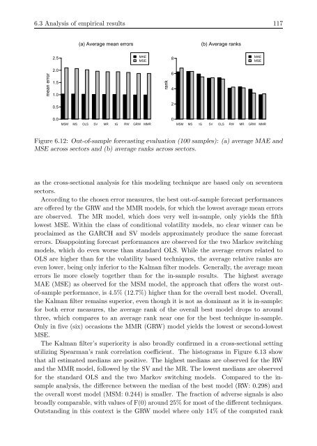
6.3 Analysis of empirical results 117 mean error 2.5 2.0 1.5 1.0 0.5 (a) Average mean errors MAE MSE 0.0 MSM MS OLS SV MR tG RW GRW MMR rank 8 6 4 2 (b) Average ranks MAE MSE 0 MSM MS tG SV OLS RW MR GRW MMR Figure 6.12: Out-of-sample forecasting evaluation (100 samples): (a) average MAE and MSE across sectors and (b) average ranks across sectors. as the cross-sectional analysis for this modeling technique are based only on seventeen sectors. According to the chosen error measures, the best out-of-sample forecast performances are offered by the GRW and the MMR models, for which the lowest average mean errors are observed. The MR model, which does very well in-sample, only yields the fifth lowest MSE. Within the class of conditional volatility models, no clear winner can be proclaimed as the GARCH and SV models approximately produce the same forecast errors. Disappointing forecast performances are observed for the two Markov switching models, which do even worse than standard OLS. While the average errors related to OLS are higher than for the volatility based techniques, the average relative ranks are even lower, being only inferior to the Kalman filter models. Generally, the average mean errors lie more closely together than for the in-sample results. The highest average MAE (MSE) as observed for the MSM model, the approach that offers the worst outof-sample performance, is 4.5% (12.7%) higher than for the overall best model. Overall, the Kalman filter remains superior, even though it is not as dominant as it is in-sample: for both error measures, the average rank of the overall best model drops to around three, which compares to an average rank near one for the best technique in-sample. Only in five (six) occasions the MMR (GRW) model yields the lowest or second-lowest MSE. The Kalman filter’s superiority is also broadly confirmed in a cross-sectional setting utilizing Spearman’s rank correlation coefficient. The histograms in Figure 6.13 show that all estimated medians are positive. The highest medians are observed for the RW and the MMR model, followed by the SV and the MR. The lowest medians are observed for the standard OLS and the two Markov switching models. Compared to the insample analysis, the difference between the median of the best model (RW: 0.298) and the overall worst model (MSM: 0.244) is smaller. The fraction of adverse signals is also broadly comparable, with values of F(0) around 25% for most of the different techniques. Outstanding in this context is the GRW model where only 14% of the computed rank
Page 1:
Sascha Mergner Applications of Stat
Page 4 and 5:
erschienen im Universitätsverlag G
Page 6 and 7:
Bibliographische Information der De
Page 9 and 10:
Contents List of figures . . . . .
Page 11 and 12:
Contents ix 4.5 Model selection and
Page 13:
Contents xi 7.5 Concluding remarks
Page 16 and 17:
xiv List of figures 6.14 Histograms
Page 19:
Notation and conventions The outlin
Page 22 and 23:
xx Used abbreviations and symbols L
Page 24 and 25:
xxii Used abbreviations and symbols
Page 26 and 27:
xxiv Used abbreviations and symbols
Page 29:
Preface The work on this book began
Page 33 and 34:
Chapter 1 Introduction “Economist
Page 35 and 36:
1.2 Research objectives 3 1.2 Resea
Page 37:
1.3 Organization of the thesis 5 to
Page 40 and 41:
8 2 Some stylized facts of weekly s
Page 42 and 43:
10 2 Some stylized facts of weekly
Page 44 and 45:
Page 46 and 47:
Page 48 and 49:
Page 50 and 51:
18 3 Linear Gaussian state space mo
Page 52 and 53:
Page 54 and 55:
Page 56 and 57:
Page 58 and 59:
Page 60 and 61:
Page 62 and 63:
Page 64 and 65:
Page 66 and 67:
Page 68 and 69:
Page 70 and 71:
Page 72 and 73:
Page 75 and 76:
Chapter 4 Markov regime switching M
Page 77 and 78:
4.1 Basic concepts 45 R t (%) 20 10
Page 79 and 80:
4.1 Basic concepts 47 probability d
Page 81 and 82:
4.3 Parameter estimation 49 X 1 X 2
Page 83 and 84:
4.3 Parameter estimation 51 4.3.2.1
Page 85 and 86:
4.4 Forecasting and decoding 53 4.4
Page 87 and 88:
4.4 Forecasting and decoding 55 mod
Page 89 and 90:
Chapter 5 Conditional heteroskedast
Page 91 and 92:
5.1 Autoregressive conditional hete
Page 93 and 94:
Page 95 and 96:
Page 97 and 98: 5.2 Stochastic volatility 65 or the
Page 99 and 100: 5.2 Stochastic volatility 67 5.2.1.
Page 101 and 102: 5.2 Stochastic volatility 69 likeli
Page 103 and 104: 5.2 Stochastic volatility 71 linear
Page 105 and 106: 5.2 Stochastic volatility 73 3. An
Page 107 and 108: 5.3 Multivariate conditional hetero
Page 113: 5.3 Multivariate conditional hetero
Page 116 and 117: 84 6 Time-varying market beta risk
Page 155 and 156: Chapter 7 A Kalman filter based con
Page 157 and 158: 7.1 Factor modeling 125 uncondition
Page 159 and 160: 7.1 Factor modeling 127 predictabil
Page 161 and 162: 7.1 Factor modeling 129 usefulness,
Page 163 and 164: 7.2 Specification of a conditional
Page 165 and 166: 7.3 The risk factors 133 Table 7.1:
Page 167 and 168: 7.3 The risk factors 135 introduced
Page 169 and 170: 7.3 The risk factors 137 auxiliary
Page 171 and 172: 7.4 Empirical results 139 Table 7.4
Page 173 and 174: 7.4 Empirical results 141 are consi
Page 177 and 178: 7.4 Empirical results 145 β TS 0.4
Page 185 and 186: 7.4 Empirical results 153 cumulativ
Page 187 and 188: Chapter 8 Conclusion and outlook Th
Page 189 and 190: Conclusion and outlook 157 cannot o
Page 191 and 192: Appendix A Brief review of asset pr
Page 193 and 194: A.3 Alternative asset pricing model
Page 195 and 196: Appendix B Figures
Page 197 and 198: Figures 165 β t β t β t 2.0 1.5
Page 199 and 200:
Figures 167 β t β t β t 2.5 2.0
Page 201 and 202:
Page 203 and 204:
Page 205 and 206:
Page 207 and 208:
Page 209 and 210:
Appendix C Tables
Page 211 and 212:
Tables 179 Table C.1 — continued
Page 213 and 214:
Tables 181 Table C.3: In-sample mea
Page 215 and 216:
Tables 183 Table C.5: Out-of-sample
Page 217 and 218:
Tables 185 Table C.7: Parameter est
Page 219 and 220:
Tables 187 Table C.7 — continued
Page 221 and 222:
Tables 189 Table C.8: Out-of-sample
Page 223 and 224:
References Abell, J. D. and T. M. K
Page 225 and 226:
References 193 Bulla, J. (2006). Ap
Page 227 and 228:
References 195 Fabozzi, F. J. and J
Page 229 and 230:
References 197 Harvey, A. C., E. Ru
Page 231 and 232:
References 199 Lie, F., R. Brooks,
Page 233 and 234:
References 201 Shephard, N. (1993).
Page 235:
State space models play a key role
show all

Applications of state space models in finance

Create successful ePaper yourself

Delete template?

Save as template?