Applications of state space models in finance
Applications of state space models in finance
Applications of state space models in finance
Create successful ePaper yourself
Turn your PDF publications into a flip-book with our unique Google optimized e-Paper software.
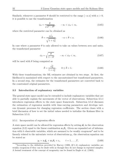
32 3 L<strong>in</strong>ear Gaussian <strong>state</strong> <strong>space</strong> <strong>models</strong> and the Kalman filter<br />
Similarly, whenever a parameter θ should be restricted to the range [−a; a] with a > 0,<br />
it is possible to use the transformation<br />
ψθ =<br />
where the restricted parameter can be obta<strong>in</strong>ed as<br />
ˆθ =<br />
θ<br />
√ a 2 − θ 2 , −∞ < ψθ < ∞, (3.65)<br />
a ˆ ψθ<br />
�<br />
1 + ˆ ψ2 , −a <<br />
θ<br />
ˆ θ < a. (3.66)<br />
In case where a parameter θ is only allowed to take on values between zero and unity,<br />
the transformed parameter<br />
�<br />
θ<br />
ψθ =<br />
1 − θ , −∞ < ψθ < ∞, (3.67)<br />
will be used with θ be<strong>in</strong>g computed as<br />
ˆθ = ˆ ψ2 θ<br />
1 + ˆ ψ2 , 0 ≤<br />
θ<br />
ˆ θ < 1. (3.68)<br />
With these transformations, the ML estimates are obta<strong>in</strong>ed <strong>in</strong> two steps. At first, the<br />
likelihood is maximized with respect to the unconstra<strong>in</strong>ed but transformed parameters.<br />
In a second step, the estimates for the transformed parameters are converted back to<br />
the constra<strong>in</strong>ed orig<strong>in</strong>al parameters.<br />
3.5 Introduction <strong>of</strong> explanatory variables<br />
The general <strong>state</strong> <strong>space</strong> model can be extended to <strong>in</strong>clude explanatory variables that are<br />
able to partially expla<strong>in</strong> the movements <strong>of</strong> the vector <strong>of</strong> observations. Subsection 3.5.1<br />
<strong>in</strong>troduces regression effects to the <strong>state</strong> <strong>space</strong> framework. Subsection 3.5.2 discusses<br />
the estimation <strong>of</strong> regression <strong>models</strong> with time-vary<strong>in</strong>g parameters and develops various<br />
dynamic processes for chang<strong>in</strong>g regression coefficients. The section closes with a<br />
brief discussion <strong>of</strong> how to set the <strong>in</strong>itial values needed to <strong>in</strong>itialize the Kalman filter <strong>in</strong><br />
Subsection 3.5.3.<br />
3.5.1 Incorporation <strong>of</strong> regression effects<br />
A <strong>state</strong> <strong>space</strong> model can be allowed for regression effects by sett<strong>in</strong>g dt <strong>in</strong> the observation<br />
equation (3.2) equal to the l<strong>in</strong>ear comb<strong>in</strong>ation xtβ t. Given an expanded set <strong>of</strong> <strong>in</strong>formation<br />
with k observable variables, which are assumed to be weakly exogenous 8 and to be<br />
l<strong>in</strong>early related to the univariate vector <strong>of</strong> observations yt, the observation equation can<br />
be <strong>state</strong>d as<br />
yt = ztξ t + xtβ t + ɛt, t = 1, . . . , T, (3.69)<br />
8 Accord<strong>in</strong>g to the def<strong>in</strong>ition provided by Harvey (1989, 7.1.4) explanatory variables are<br />
weakly exogenous if they can be dealt with as though they do not change <strong>in</strong> repeated samples.<br />
A formal treatment <strong>of</strong> the concept <strong>of</strong> exogeneity can be found <strong>in</strong> Engle et al. (1983).


