Applications of state space models in finance

More documents

Recommendations

Info

66 5 Conditional heteroskedasticity models via simulation-based techniques. In this regard, the SV model turns out to be strongly connected to the state space framework outlined in Chapter 3. Subsection 5.2.1 introduces a representation for the univariate case, deals with the difficulties related to the estimation of SV models and summarizes the basic statistical properties of the model. Subection 5.2.2 gives an overview of the major procedures for statistical inference discussed in the literature. In Subection 5.2.3, the main ideas behind Monte Carlo likelihood, the estimation framework that will be used throughout this thesis for estimation purposes, will be highlighted. The final subsection contains a brief overview of possible extensions of the basic SV model. 5.2.1 The basic stochastic volatility model Following Ghysels et al. (1996) the basic SV models in discrete time for a univariate time series yt of asset log-returns can be written as: � 1 yt = µ + σ∗ exp 2 ht � ɛt, ɛt ∼ IID(0, 1), (5.25) with ht+1 = φht + ηt, ηt ∼ IID � 0, σ 2� η , h1 ∼ N � 0, σ 2 η/(1 − φ 2 ) � , (5.26) for t = 1, . . . , T . The parameter µ denotes the unconditional expectation of the return process yt. The scaling parameter σ∗ is the average standard deviation with σ∗ > 0. The unobserved log-volatility process is denoted by ht = log � σ2 � t . As in the case of . The the EGARCH model (cf. ¢ 5.1.2) the use of logarithms ensures positivity of σ2 t persistence parameter φ with 0 < φ < 1, plays a similar role as the sum γ1 + δ1 for the GARCH(1,1) model. The parameter usually takes on values greater than 0.8. As most financial time series exhibit no pronounced serial dependence in the mean equation, the constant µ will be treated as fixed and set to zero in the following. 14 Although ht can be modeled by any stationary autoregressive process, it is common to choose a first-order autoregressive process. The disturbances ɛt and ηt are Gaussian white noise. They are assumed to be uncorrelated, contemporaneously and at all lags. Franses and van Dijk (2000, ¢ 4.1.1) offer a useful interpretation of the two different shocks: ɛt represents the contents of new information (good or bad news); ηt reflects the shocks to the newsflow’s intensity. The SV model in (5.25) and (5.26) is commonly referred to as the log-normal SV model. It represents a state space model where the observation equation describes the relationship between the univariate vector of observations, y = (y1, . . . , yT ) ′ , and the state vector. The latent volatility process θ = (h1, . . . , hT ) ′ is specified in the state equation, which models the dynamic properties of ht. As ɛt and ht, which both enter the multiplication in the mean equation, are stochastic, the basic SV model is nonlinear. The Kalman filter as introduced in ¢ 3.3 cannot be applied directly for estimation purposes. 14 Alternatively, some authors prefer to use mean-corrected returns y ∗ t := log(Pt) − log(Pi,t−1) − (1/T ) �T i=0 (log(Pt) − log(Pi,t−1)), see, for example, Kim et al. (1998).
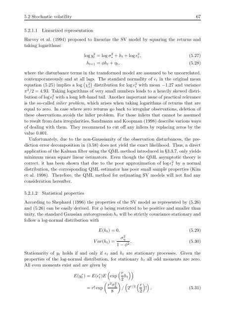
5.2 Stochastic volatility 67 5.2.1.1 Linearized representation Harvey et al. (1994) proposed to linearize the SV model by squaring the returns and taking logarithms: log y 2 t = log σ2 ∗ + ht + log ɛ 2 t , (5.27) ht+1 = φht + ηt, (5.28) where the disturbance terms in the transformed model are assumed to be uncorrelated, contemporaneously and at all lags. The standard normality of ɛt in the original mean equation (5.25) implies a log � χ2 � 2 1 distribution for log ɛt with mean −1.27 and variance π 2 /2 = 4.93. Taking logarithms of very small numbers leads to a heavily skewed distribution of log ɛ 2 t with a long left-hand tail. Another important issue of practical relevance is the so-called inlier problem, which arises when taking logarithms of returns that are equal to zero. In case where zero returns go back to irregular observations, deletion of these observations avoids the inlier problem. For those inliers that cannot be assumed to result from data irregularities, Sandmann and Koopman (1998) describe various ways of dealing with them. They recommend to cut off any inliers by replacing zeros by the value 0.001. Unfortunately, due to the non-Gaussianity of the observation disturbances, the prediction error decomposition in (3.58) does not yield the exact likelihood. Thus, a direct application of the Kalman filter using the QML method introduced in ¢ 3.3.7, only yields minimum mean square linear estimators. Even though the QML asymptotic theory is correct, it has been shown that due to the poor approximation of log ɛ2 t by a normal distribution, the corresponding QML estimator has poor small sample properties (Kim et al. 1998). Therefore, the QML method for estimating SV models will not find any consideration hereafter. 5.2.1.2 Statistical properties According to Shephard (1996) the properties of the SV model as represented by (5.26) and (5.26) can be easily derived. For φ being restricted to be positive and smaller than unity, the standard Gaussian autoregression ht will be strictly covariance stationary and follow a log-normal distribution with E(ht) = 0, (5.29) V ar(ht) = σ2 η . (5.30) 1 − φ2 Stationarity of yt holds if and only if ɛt and ht are stationary processes. Given the properties of the log-normal distribution, for stationary ht all odd moments are zero. All even moments exist and are given by E(y r t ) = E(ɛ r � � r t )E exp 2 ht �� 2 2 r σ � h = r! exp / 8 2 r/2 � r 2 � � ! , (5.31)
Page 1:
Sascha Mergner Applications of Stat
Page 4 and 5:
erschienen im Universitätsverlag G
Page 6 and 7:
Bibliographische Information der De
Page 9 and 10:
Contents List of figures . . . . .
Page 11 and 12:
Contents ix 4.5 Model selection and
Page 13:
Contents xi 7.5 Concluding remarks
Page 16 and 17:
xiv List of figures 6.14 Histograms
Page 19:
Notation and conventions The outlin
Page 22 and 23:
xx Used abbreviations and symbols L
Page 24 and 25:
xxii Used abbreviations and symbols
Page 26 and 27:
xxiv Used abbreviations and symbols
Page 29:
Preface The work on this book began
Page 33 and 34:
Chapter 1 Introduction “Economist
Page 35 and 36:
1.2 Research objectives 3 1.2 Resea
Page 37:
1.3 Organization of the thesis 5 to
Page 40 and 41:
8 2 Some stylized facts of weekly s
Page 42 and 43:
10 2 Some stylized facts of weekly
Page 44 and 45:
Page 46 and 47:
Page 48 and 49: 16 2 Some stylized facts of weekly
Page 50 and 51: 18 3 Linear Gaussian state space mo
Page 75 and 76: Chapter 4 Markov regime switching M
Page 77 and 78: 4.1 Basic concepts 45 R t (%) 20 10
Page 79 and 80: 4.1 Basic concepts 47 probability d
Page 81 and 82: 4.3 Parameter estimation 49 X 1 X 2
Page 83 and 84: 4.3 Parameter estimation 51 4.3.2.1
Page 85 and 86: 4.4 Forecasting and decoding 53 4.4
Page 87 and 88: 4.4 Forecasting and decoding 55 mod
Page 89 and 90: Chapter 5 Conditional heteroskedast
Page 91 and 92: 5.1 Autoregressive conditional hete
Page 97: 5.2 Stochastic volatility 65 or the
Page 101 and 102: 5.2 Stochastic volatility 69 likeli
Page 103 and 104: 5.2 Stochastic volatility 71 linear
Page 105 and 106: 5.2 Stochastic volatility 73 3. An
Page 107 and 108: 5.3 Multivariate conditional hetero
Page 113: 5.3 Multivariate conditional hetero
Page 116 and 117: 84 6 Time-varying market beta risk
Page 148 and 149:
116 6 Time-varying market beta risk
Page 150 and 151:
Page 152 and 153:
Page 155 and 156:
Chapter 7 A Kalman filter based con
Page 157 and 158:
7.1 Factor modeling 125 uncondition
Page 159 and 160:
7.1 Factor modeling 127 predictabil
Page 161 and 162:
7.1 Factor modeling 129 usefulness,
Page 163 and 164:
7.2 Specification of a conditional
Page 165 and 166:
7.3 The risk factors 133 Table 7.1:
Page 167 and 168:
7.3 The risk factors 135 introduced
Page 169 and 170:
7.3 The risk factors 137 auxiliary
Page 171 and 172:
7.4 Empirical results 139 Table 7.4
Page 173 and 174:
7.4 Empirical results 141 are consi
Page 175 and 176:
Page 177 and 178:
7.4 Empirical results 145 β TS 0.4
Page 179 and 180:
Page 181 and 182:
Page 183 and 184:
Page 185 and 186:
7.4 Empirical results 153 cumulativ
Page 187 and 188:
Chapter 8 Conclusion and outlook Th
Page 189 and 190:
Conclusion and outlook 157 cannot o
Page 191 and 192:
Appendix A Brief review of asset pr
Page 193 and 194:
A.3 Alternative asset pricing model
Page 195 and 196:
Appendix B Figures
Page 197 and 198:
Figures 165 β t β t β t 2.0 1.5
Page 199 and 200:
Page 201 and 202:
Page 203 and 204:
Page 205 and 206:
Page 207 and 208:
Page 209 and 210:
Appendix C Tables
Page 211 and 212:
Tables 179 Table C.1 — continued
Page 213 and 214:
Tables 181 Table C.3: In-sample mea
Page 215 and 216:
Tables 183 Table C.5: Out-of-sample
Page 217 and 218:
Tables 185 Table C.7: Parameter est
Page 219 and 220:
Tables 187 Table C.7 — continued
Page 221 and 222:
Tables 189 Table C.8: Out-of-sample
Page 223 and 224:
References Abell, J. D. and T. M. K
Page 225 and 226:
References 193 Bulla, J. (2006). Ap
Page 227 and 228:
References 195 Fabozzi, F. J. and J
Page 229 and 230:
References 197 Harvey, A. C., E. Ru
Page 231 and 232:
References 199 Lie, F., R. Brooks,
Page 233 and 234:
References 201 Shephard, N. (1993).
Page 235:
State space models play a key role
show all

Applications of state space models in finance

Create successful ePaper yourself

Delete template?

Save as template?