- Page 1 and 2:
A Guide to LAT E X and Electronic P
- Page 3:
Trademark notices METAFONT is a tra
- Page 6 and 7:
viii Preface example, the section o
- Page 8 and 9:
x CONTENTS 4.6 Tabulator stops . .
- Page 10 and 11:
xii CONTENTS B The L AT E X Clockwo
- Page 12 and 13:
xiv CONTENTS H.22 A M S Greek and H
- Page 15 and 16:
1 1.1 Just what is L AT E X? To sum
- Page 17 and 18:
He took a {\bf bold step} forward.
- Page 19 and 20:
1.3. T E X and its offspring 7 Alth
- Page 21 and 22:
1.3. T E X and its offspring 9 Font
- Page 23 and 24:
1.5. Basics of a L AT E X file 11 v
- Page 25 and 26:
1.5. Basics of a L AT E X file 13 c
- Page 27 and 28:
1.6. T E X processing procedure 15
- Page 29 and 30:
2 Text, Symbols, and Commands The t
- Page 31 and 32:
2.2. Environments 19 a punctuation
- Page 33 and 34:
2.4. Lengths 21 Declarations made w
- Page 35 and 36:
2.5. Special characters 23 Instead
- Page 37 and 38:
2.5. Special characters 25 which de
- Page 39 and 40:
2.5.11 The date 2.6. Exercises 27 T
- Page 41 and 42:
2.7. Fine-tuning text 29 simply a s
- Page 43 and 44:
2.7. Fine-tuning text 31 Any combin
- Page 45 and 46:
\bigskip \medskip \smallskip 2.7. F
- Page 47 and 48:
2.8. Word division 35 that works (a
- Page 49 and 50:
3 3.1 Document class Document Layou
- Page 51 and 52:
3.1. Document class 39 pages and on
- Page 53 and 54:
3.1. Document class 41 space betwee
- Page 55 and 56:
The command \thispagestyle{style} 3
- Page 57 and 58:
3.2. Page style 45 In many classes,
- Page 59 and 60:
3.2. Page style 47 There is a recen
- Page 61 and 62:
3.2. Page style 49 forget the 1 inc
- Page 63 and 64:
3.2. Page style 51 As you see, the
- Page 65 and 66:
\title{% How to Write DVI Drivers}
- Page 67 and 68:
3.3.2 Abstract The abstract is prod
- Page 69 and 70:
3.3. Parts of the document 57 (The
- Page 71 and 72:
3.4. Table of contents 59 given at
- Page 73 and 74:
4 Displayed Text There are a variet
- Page 75 and 76:
\tiny smallest \scriptsize very sma
- Page 77 and 78:
4.1. Changing font 65 that a font e
- Page 79 and 80:
4.2 Centering and indenting 4.2.1 C
- Page 81 and 82:
4.3 Lists 4.3. Lists 69 Exercise 4.
- Page 83 and 84:
4.3. Lists 71 The \item[option] com
- Page 85 and 86:
4.3. Lists 73 label. For the enumer
- Page 87 and 88:
4.4. Generalized lists 75 However,
- Page 89 and 90:
4.4. Generalized lists 77 normally
- Page 91 and 92:
4.4. Generalized lists 79 item are
- Page 93 and 94:
4.6. Tabulator stops 81 which also
- Page 95 and 96:
4.6.4 Further tabbing commands 4.6.
- Page 97 and 98:
4.7. Boxes 85 tentative 2004 = $100
- Page 99 and 100:
4.7. Boxes 87 To make a framed box
- Page 101 and 102:
This is a 3.5 cm wide parbox. It is
- Page 103 and 104:
4.7. Boxes 91 The optional argument
- Page 105 and 106:
4.7. Boxes 93 contents as a unit wi
- Page 107 and 108:
4.8. Tables 95 This package also al
- Page 109 and 110:
4.8. Tables 97 If the left or right
- Page 111 and 112: 4.8. Tables 99 Position Club Games
- Page 113 and 114: 4.8. Tables 101 4 & Daysdon Bombers
- Page 115 and 116: 4.8. Tables 103 The \raisebox comma
- Page 117 and 118: 4.8. Tables 105 terminate the row i
- Page 119 and 120: 4.8. Tables 107 Package: The array
- Page 121 and 122: Primary Energy Consumption 4.8. Tab
- Page 123 and 124: 4.9. Printing literal text 111 \ver
- Page 125 and 126: 4.10. Footnotes and marginal notes
- Page 127 and 128: 4.10. Footnotes and marginal notes
- Page 129 and 130: 4.10. Footnotes and marginal notes
- Page 131 and 132: 5 Mathematical Formulas Mathematics
- Page 133 and 134: 5.2. Main elements of math mode 121
- Page 135 and 136: 5.2.5 Sums and integrals 5.2. Main
- Page 137 and 138: 5.3.1 Greek letters 5.3. Mathematic
- Page 139 and 140: 5.3. Mathematical symbols 127 < \no
- Page 141 and 142: 5.3. Mathematical symbols 129 Some
- Page 143 and 144: 5.4. Additional elements 131 articl
- Page 145 and 146: 5.4.2 Ordinary text within a formul
- Page 147 and 148: 5.4. Additional elements 135 \[ \su
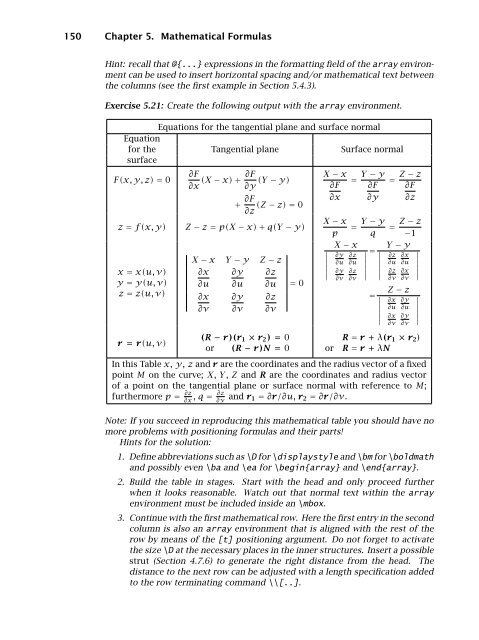
- Page 149 and 150: 123 a + b + · · · + y +z
- Page 151 and 152: left formula & mid formula & right
- Page 153 and 154: 5.4. Additional elements 141 Exerci
- Page 155 and 156: 5.4. Additional elements 143 5.4.9
- Page 157 and 158: 5.5 Fine-tuning mathematics 5.5.1 H
- Page 159 and 160: a0 + a1 + 1 a2 + 1 1 a3 + 1 a4 5.5.
- Page 161: 5.5. Fine-tuning mathematics 149 \a
- Page 166 and 167: 154 Chapter 6. Graphics Inclusion a
- Page 168 and 169: 156 Chapter 6. Graphics Inclusion a
- Page 170 and 171: 158 Chapter 6. Graphics Inclusion a
- Page 172 and 173: 160 Chapter 6. Graphics Inclusion a
- Page 174 and 175: 162 Chapter 6. Graphics Inclusion a
- Page 176 and 177: 164 Chapter 6. Graphics Inclusion a
- Page 178 and 179: 166 Chapter 6. Graphics Inclusion a
- Page 180 and 181: 168 Chapter 6. Graphics Inclusion a
- Page 182 and 183: 170 Chapter 7. Floating tables and
- Page 184 and 185: 172 Chapter 7. Floating tables and
- Page 186 and 187: 174 Chapter 7. Floating tables and
- Page 188 and 189: 176 Chapter 7. Floating tables and
- Page 190 and 191: 178 Chapter 7. Floating tables and
- Page 192 and 193: 180 Chapter 7. Floating tables and
- Page 194 and 195: 182 Chapter 8. User Customizations
- Page 196 and 197: 184 Chapter 8. User Customizations
- Page 198 and 199: 186 Chapter 8. User Customizations
- Page 200 and 201: 188 Chapter 8. User Customizations
- Page 202 and 203: 190 Chapter 8. User Customizations
- Page 204 and 205: 192 Chapter 8. User Customizations
- Page 206 and 207: 194 Chapter 8. User Customizations
- Page 208 and 209: 196 Chapter 8. User Customizations
- Page 210 and 211: 198 Chapter 8. User Customizations
- Page 212 and 213:
200 Chapter 8. User Customizations
- Page 214 and 215:
202 Chapter 8. User Customizations
- Page 216 and 217:
204 Chapter 8. User Customizations
- Page 219 and 220:
9 Document Management This chapter
- Page 221 and 222:
9.1. Processing parts of a document
- Page 223 and 224:
9.1.3 Monitor input and output 9.1.
- Page 225 and 226:
9.2 In-text references 9.2. In-text
- Page 227 and 228:
9.2. In-text references 215 can be
- Page 229 and 230:
9.3. Bibliographies 217 by means of
- Page 231 and 232:
9.3. Bibliographies 219 by the last
- Page 233 and 234:
\bibitem [short(year)long] {key} .
- Page 235 and 236:
9.3. Bibliographies 223 sectionbib
- Page 237 and 238:
9.4 Keyword index 9.4. Keyword inde
- Page 239 and 240:
9.4. Keyword index 227 An entry may
- Page 241 and 242:
9.4. Keyword index 229 number of op
- Page 243 and 244:
10 PostScript and PDF PostScript is
- Page 245 and 246:
10.1. L AT E X and PostScript 233 A
- Page 247 and 248:
10.1. L AT E X and PostScript 235 T
- Page 249 and 250:
10.2. Portable Document Format 237
- Page 251 and 252:
10.2. Portable Document Format 239
- Page 253 and 254:
10.2. Portable Document Format 241
- Page 255 and 256:
10.2. Portable Document Format 243
- Page 257 and 258:
10.2. Portable Document Format 245
- Page 259 and 260:
10.2. Portable Document Format 247
- Page 261:
10.2. Portable Document Format 249
- Page 264 and 265:
252 Chapter 11. Multilingual L AT E
- Page 266 and 267:
254 Chapter 11. Multilingual L AT E
- Page 268 and 269:
256 Chapter 11. Multilingual L AT E
- Page 270 and 271:
258 Chapter 12. Math Extensions wit
- Page 272 and 273:
260 Chapter 12. Math Extensions wit
- Page 274 and 275:
262 Chapter 12. Math Extensions wit
- Page 276 and 277:
264 Chapter 12. Math Extensions wit
- Page 278 and 279:
266 Chapter 12. Math Extensions wit
- Page 280 and 281:
268 Chapter 12. Math Extensions wit
- Page 282 and 283:
270 Chapter 12. Math Extensions wit
- Page 284 and 285:
272 Chapter 12. Math Extensions wit
- Page 286 and 287:
274 Chapter 12. Math Extensions wit
- Page 288 and 289:
276 Chapter 12. Math Extensions wit
- Page 290 and 291:
278 Chapter 12. Math Extensions wit
- Page 292 and 293:
280 Chapter 12. Math Extensions wit
- Page 294 and 295:
282 Chapter 12. Math Extensions wit
- Page 296 and 297:
284 Chapter 12. Math Extensions wit
- Page 299 and 300:
13 Drawing with LAT E X The inclusi
- Page 301 and 302:
13.1. The picture environment 289 w
- Page 303 and 304:
Picture boxes—rectangles 13.1. Th
- Page 305 and 306:
13.1. The picture environment 293 T
- Page 307 and 308:
\vector(∆x,∆y){length} 13.1. Th
- Page 309 and 310:
13.1. The picture environment 297 d
- Page 311 and 312:
\frame{pic elem} 13.1. The picture
- Page 313 and 314:
13.1. The picture environment 301 T
- Page 315 and 316:
13.2. Extended pictures 303 \matrix
- Page 317 and 318:
13.2. Extended pictures 305 The def
- Page 319 and 320:
13.3 Other drawing packages 13.3.1
- Page 321 and 322:
14 Bibliographic Databases and BIBT
- Page 323 and 324:
14.2. Creating a bibliographic data
- Page 325 and 326:
14.2. Creating a bibliographic data
- Page 327 and 328:
14.2. Creating a bibliographic data
- Page 329 and 330:
14.2. Creating a bibliographic data
- Page 331 and 332:
14.2. Creating a bibliographic data
- Page 333 and 334:
} note = {} 14.3. Customizing bibli
- Page 335 and 336:
15 Presentation Material So far we
- Page 337 and 338:
as \documentclass{slides} preamble
- Page 339 and 340:
15.1. Slide production with SLIT E
- Page 341 and 342:
15.1. Slide production with SLIT E
- Page 343 and 344:
15.2. Slide production with seminar
- Page 345 and 346:
15.2. Slide production with seminar
- Page 347 and 348:
15.2. Slide production with seminar
- Page 349 and 350:
15.2. Slide production with seminar
- Page 351 and 352:
Local configuration 15.2. Slide pro
- Page 353 and 354:
15.3. Electronic documents for scre
- Page 355 and 356:
15.4. Special effects with PDF 343
- Page 357 and 358:
Package: background \Replace pages
- Page 359 and 360:
15.4. Special effects with PDF 347
- Page 361:
15.4. Special effects with PDF 349
- Page 364 and 365:
352 Chapter 16. Letters in the prea
- Page 366 and 367:
354 Chapter 16. Letters A sample le
- Page 368 and 369:
356 Chapter 16. Letters without a c
- Page 370 and 371:
358 Chapter 16. Letters properly po
- Page 372 and 373:
360 Chapter 16. Letters \DeclareOpt
- Page 374 and 375:
362 Chapter 16. Letters {\viiisf\un
- Page 376 and 377:
364 Chapter 16. Letters \ifthenelse
- Page 379 and 380:
A The New Font Selection Scheme (NF
- Page 381 and 382:
A.1. Font attributes under NFSS 369
- Page 383 and 384:
A.2. Simplified font selection 371
- Page 385 and 386:
A.3.2 Defining font commands A.3. I
- Page 387 and 388:
A.3. Installing fonts with NFSS 375
- Page 389 and 390:
A.3. Installing fonts with NFSS 377
- Page 391 and 392:
\renewcommand{\rmdefault}{ptm} \ren
- Page 393 and 394:
B The LAT E X Clockwork In this app
- Page 395 and 396:
Figure B.1: The T E XLive welcome B
- Page 397 and 398:
B.1. Installing L AT E X 385 fontte
- Page 399 and 400:
B.2 Obtaining the Adobe euro fonts
- Page 401 and 402:
B.4. The CTAN server 389 dvipdfm (S
- Page 403 and 404:
B.5 Additional standard files B.5.
- Page 405 and 406:
B.5. Additional standard files 393
- Page 407 and 408:
B.5. Additional standard files 395
- Page 409 and 410:
B.6. The various L AT E X files 397
- Page 411 and 412:
B.6. The various L AT E X files 399
- Page 413 and 414:
C Error Messages Errors are bound t
- Page 415 and 416:
C.1. Basic structure of error messa
- Page 417 and 418:
C.1. Basic structure of error messa
- Page 419 and 420:
C.1. Basic structure of error messa
- Page 421 and 422:
C.2 Some sample errors C.2.1 Error
- Page 423 and 424:
C.2. Some sample errors 411 The las
- Page 425 and 426:
C.2. Some sample errors 413 message
- Page 427 and 428:
C.3. List of L AT E X error message
- Page 429 and 430:
C.3. List of L AT E X error message
- Page 431 and 432:
! LaTeX Error: No \title given. C.3
- Page 433 and 434:
C.3.2 L AT E X package errors C.3.
- Page 435 and 436:
C.3. List of L AT E X error message
- Page 437 and 438:
! Extra alignment tab has been chan
- Page 439 and 440:
C.4. T E X error messages 427 the t
- Page 441 and 442:
C.5. Warnings 429 the result of an
- Page 443 and 444:
LaTeX Warning: No \author given. C.
- Page 445 and 446:
C.5.3 L AT E X font warnings C.5. W
- Page 447 and 448:
C.6. Search for subtle errors 435 b
- Page 449 and 450:
D LAT E X Programming In this appen
- Page 451 and 452:
D.1. Class and package files 439 \p
- Page 453 and 454:
l.1 \NeedsTeXFormat {LaTeX2e} D.2.
- Page 455 and 456:
D.2. L AT E X programming commands
- Page 457 and 458:
D.2. L AT E X programming commands
- Page 459 and 460:
D.2. L AT E X programming commands
- Page 461 and 462:
\begin{filecontents}{mymacros} \new
- Page 463 and 464:
\noexpand \expandafter D.3. Sample
- Page 465 and 466:
D.3. Sample packages 453 \setboolea
- Page 467 and 468:
D.3. Sample packages 455 \newcomman
- Page 469 and 470:
D.3. Sample packages 457 sec-name:
- Page 471 and 472:
The priest fulfills several functio
- Page 473 and 474:
\ifcase command (page 451). D.5. Di
- Page 475 and 476:
D.7. Managing code and documentatio
- Page 477 and 478:
D.7. Managing code and documentatio
- Page 479 and 480:
D.7. Managing code and documentatio
- Page 481 and 482:
\StopEventually{final text} D.7. Ma
- Page 483 and 484:
Integrity tests D.7. Managing code
- Page 485:
D.7. Managing code and documentatio
- Page 488 and 489:
476 Appendix E. L AT E X and World
- Page 490 and 491:
478 Appendix E. L AT E X and World
- Page 492 and 493:
480 Appendix E. L AT E X and World
- Page 494 and 495:
482 Appendix E. L AT E X and World
- Page 496 and 497:
484 Appendix F. Obsolete L AT E X r
- Page 498 and 499:
486 Appendix F. Obsolete L AT E X t
- Page 500 and 501:
488 Appendix G. T E X Fonts or for
- Page 502 and 503:
490 Appendix G. T E X Fonts A book
- Page 504 and 505:
492 Appendix G. T E X Fonts 0 1 2 3
- Page 506 and 507:
494 Appendix G. T E X Fonts Package
- Page 508 and 509:
496 Appendix G. T E X Fonts 0 1 2 3
- Page 510 and 511:
498 Appendix G. T E X Fonts The pri
- Page 512 and 513:
500 Appendix G. T E X Fonts 0 1 2 3
- Page 514 and 515:
502 Appendix G. T E X Fonts 0 1 2 3
- Page 516 and 517:
504 Appendix G. T E X Fonts own. Th
- Page 518 and 519:
506 Appendix G. T E X Fonts viewing
- Page 520 and 521:
508 Appendix H. Command Summary " .
- Page 522 and 523:
510 Appendix H. Command Summary \<
- Page 524 and 525:
512 Appendix H. Command Summary \a=
- Page 526 and 527:
514 Appendix H. Command Summary \ap
- Page 528 and 529:
516 Appendix H. Command Summary \be
- Page 530 and 531:
518 Appendix H. Command Summary \be
- Page 532 and 533:
520 Appendix H. Command Summary whi
- Page 534 and 535:
522 Appendix H. Command Summary \be
- Page 536 and 537:
524 Appendix H. Command Summary \be
- Page 538 and 539:
526 Appendix H. Command Summary \bm
- Page 540 and 541:
528 Appendix H. Command Summary \ch
- Page 542 and 543:
530 Appendix H. Command Summary \co
- Page 544 and 545:
532 Appendix H. Command Summary \db
- Page 546 and 547:
534 Appendix H. Command Summary \De
- Page 548 and 549:
536 Appendix H. Command Summary \De
- Page 550 and 551:
538 Appendix H. Command Summary \dh
- Page 552 and 553:
540 Appendix H. Command Summary \em
- Page 554 and 555:
542 Appendix H. Command Summary \fb
- Page 556 and 557:
544 Appendix H. Command Summary \fo
- Page 558 and 559:
546 Appendix H. Command Summary \gr
- Page 560 and 561:
548 Appendix H. Command Summary \hu
- Page 562 and 563:
550 Appendix H. Command Summary \in
- Page 564 and 565:
552 Appendix H. Command Summary \it
- Page 566 and 567:
554 Appendix H. Command Summary \le
- Page 568 and 569:
556 Appendix H. Command Summary \li
- Page 570 and 571:
558 Appendix H. Command Summary \Ma
- Page 572 and 573:
560 Appendix H. Command Summary \md
- Page 574 and 575:
562 Appendix H. Command Summary \ne
- Page 576 and 577:
564 Appendix H. Command Summary \no
- Page 578 and 579:
566 Appendix H. Command Summary \op
- Page 580 and 581:
568 Appendix H. Command Summary \pa
- Page 582 and 583:
570 Appendix H. Command Summary \pa
- Page 584 and 585:
572 Appendix H. Command Summary \Pr
- Page 586 and 587:
574 Appendix H. Command Summary \re
- Page 588 and 589:
576 Appendix H. Command Summary \ro
- Page 590 and 591:
578 Appendix H. Command Summary \se
- Page 592 and 593:
580 Appendix H. Command Summary \si
- Page 594 and 595:
582 Appendix H. Command Summary \su
- Page 596 and 597:
584 Appendix H. Command Summary \te
- Page 598 and 599:
586 Appendix H. Command Summary \te
- Page 600 and 601:
588 Appendix H. Command Summary top
- Page 602 and 603:
590 Appendix H. Command Summary \un
- Page 604 and 605:
592 Appendix H. Command Summary \va
- Page 606 and 607:
594 Appendix H. Command Summary \wi
- Page 608 and 609:
596 Appendix H. Command Summary Tab
- Page 610 and 611:
598 Appendix H. Command Summary Tab
- Page 612 and 613:
600 Appendix H. Command Summary Tab
- Page 614 and 615:
602 Appendix H. Command Summary ✲
- Page 616 and 617:
604 Appendix H. Command Summary Rem
- Page 618 and 619:
606 BIBLIOGRAPHY Knuth D. E. (1986e
- Page 620 and 621:
608 INDEX \= (¯ accent), 24, 510 \
- Page 622 and 623:
610 INDEX \Hat, 263, 546 \hdotsfor,
- Page 624 and 625:
612 INDEX creating, 311 cross-refer
- Page 626 and 627:
614 INDEX \chi, 125, 528 chicago pa
- Page 628 and 629:
616 INDEX \dbltextfloatsep, 172, 53
- Page 630 and 631:
618 INDEX e.tex, 394, 413 EC fonts,
- Page 632 and 633:
620 INDEX \exp, 128, 541 \expandaft
- Page 634 and 635:
622 INDEX cmr10 (standard), 492 cms
- Page 636 and 637:
624 INDEX Gaulle, Bernard, 251 \gcd
- Page 638 and 639:
626 INDEX initex, 6, 251, 253, 256,
- Page 640 and 641:
628 INDEX L AT E X standard, 351-6
- Page 642 and 643:
630 INDEX \mathscr, 284 \mathsf, 13
- Page 644 and 645:
632 INDEX \oint, 128, 565 \Omega, 1
- Page 646 and 647:
634 INDEX two-column, 38, 51 two-si
- Page 648 and 649:
636 INDEX plain page style, 42, 45,
- Page 650 and 651:
638 INDEX \rightharpoondown, 127, 5
- Page 652 and 653:
640 INDEX slide environment (slides
- Page 654 and 655:
642 INDEX column repetition, 96 col
- Page 656 and 657:
644 INDEX \texttt, 65, 88, 372, 585
- Page 658:
646 INDEX \varrho, 125, 591 \varsig