TESTING INTERNATIONAL PRICE TRANSMISSION UNDER ...
TESTING INTERNATIONAL PRICE TRANSMISSION UNDER ...
TESTING INTERNATIONAL PRICE TRANSMISSION UNDER ...

You also want an ePaper? Increase the reach of your titles
YUMPU automatically turns print PDFs into web optimized ePapers that Google loves.
∆p<br />
+<br />
t<br />
∑<br />
⎡β⎤<br />
' ⎡ p t<br />
= α⎢<br />
µ<br />
⎥ ⎢<br />
⎣ ⎦ ⎣tE<br />
d<br />
m=<br />
1<br />
Θ<br />
m<br />
w<br />
m, t<br />
−1<br />
t−1<br />
+ ε<br />
⎤<br />
⎥ + γE<br />
⎦<br />
t<br />
t<br />
+<br />
∑<br />
k−1<br />
i=<br />
1<br />
Γ ∆p<br />
i<br />
t−i<br />
Empirical Tests for Spatial Price Analysis<br />
+<br />
∑<br />
k<br />
i=<br />
1<br />
∑<br />
q<br />
j=<br />
2<br />
k<br />
i, j<br />
D<br />
j, t+<br />
k −i<br />
+<br />
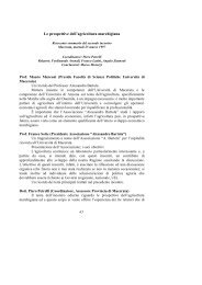
(3.41)<br />
where k is the lag length of the underlying VAR. Et is a vector of q dummy<br />
variables that take the value 1, i.e E = 1.,<br />
if the observation belongs to the j th<br />
jt<br />
36<br />
period (j = 1, … q), and 0 otherwise; that is, E t = [ E1t<br />
E2t<br />
... Eqt<br />
]' . Dt is an<br />
impulse dummy (with its lagged values) that equals unity if the observation t is<br />
the i th of the j th period, and is included to allow the conditional likelihood function<br />
to be derived given the initial values in each period (for example, if k = 3, impulse<br />
dummies will thereby have the value 1 at t+2, t+1, t, where t is the first<br />
observation of each period); wt are intervention dummies (up to d) included in<br />
order to render the residuals well behaved. The short run parameters are γ (2 X q),<br />
Γ (2 X 2), k (2 X 1) for each j and i, and Θ (2 X 2). εt are assumed to be i.i.d. with<br />
zero mean and symmetric and positive definite variance, Ω.<br />
µ = [ μ1t<br />
μ2t<br />
... μqt<br />
]' is the vector containing the long run drift parameters and<br />
β are the long run coefficients in the cointegrating vector. The cointegration<br />
⎡β⎤<br />
'<br />
hypothesis is formulated by testing the rank of π = α⎢<br />
⎥ ; its asymptotic<br />
⎣µ<br />
⎦<br />
distribution depends on the number of non-stationary relations, the location of<br />
breakpoints and the trend specification.<br />
It should be noticed that this framework includes two models: a first one is<br />
where there are no linear trends in the levels of the endogenous variables and the<br />
first differenced series have a zero mean; the broken level is restricted to the<br />
cointegration space (i.e., γ = 0, and the regime dummies are not multiplied by any<br />
trend in the cointegration vector). In the second case, a broken linear trend is<br />
accounted for in the cointegration vector but any long run linear growth is not<br />
accounted for by the model (i.e., γ ≠0 and t ≠ 0 in the cointegration vector).<br />
An application of the Johansen, Mosconi and Nielsen procedure to agricultural<br />
future and export prices is presented in Dawson et al. (2006) and Dawson and<br />
Sanjuan (2006), and will be used for the empirical analysis in chapter 6 since, as it<br />
will be clear, structural breaks can be a mean of representing the changes in policy<br />
regimes while testing for price transmission.<br />
36 '<br />
For example, if q = 3, i.e. there are two structural breaks, we have t [ E E E ] = [ 1 0 0]<br />
the observations of time t belong to the first period, '<br />
t = [ 0 1 0]<br />
' and E t = [ 0 0 1]<br />
otherwise.<br />
E if<br />
= 1 , t 2,<br />
t 3,<br />
t<br />
E if they belong to the second one,<br />
47