TESTING INTERNATIONAL PRICE TRANSMISSION UNDER ...

Empirical Analysis: Cointegration Models Accounting for Policy Regime Changes
α
LM test
ARCH(13)
84
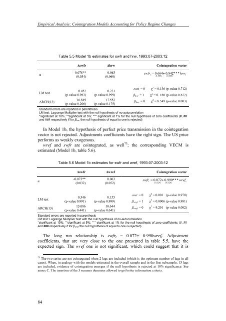
Table 5.5 Model 1b estimates for swfr and hrw, 1993:07-2003:12
∆swfr ∆hrw Cointegration vector
-0.078**
(0.034)
0.452
(p-value 0.963)
16.849
(p-value 0.206)
0.063
(0.060)
0.221
(p-value 0.999)
17.552
(p-value 0.175)
swfr = 0.
664+
0.
842*
* * hrw
t
( 1.
505)
( 0.
305)
cost = 0 χ 2 = 0.136 (p-value 0.712)
β hwr = 1 χ 2 = 0. 180 (p-value 0.672)
β hwr = 0 χ 2 = 8.549 (p-value 0.003)
Standard errors are reported in parenthesis
LM test: Lagrange Multiplier test with the null hypothesis of no-autocorrelation
*significant at 10%; **significant at 5%; *** significant at 1% for the null hypothesis of zero coefficients (#, ##
and ### respectively if for βhrw the null hypothesis of equal to one is rejected)
In Model 1b, the hypothesis of perfect price transmission in the cointegration
vector is not rejected. Adjustments coefficients have the right sign. The US price
performs as weakly exogenous.
wref and swfr are cointegrated, as well 73 ; the corresponding VECM is
estimated (Model 1b, table 5.6).
α
LM test
ARCH(13)
Table 5.6 Model 1b estimates for swfr and wref, 1993:07-2003:12
∆swfr ∆wref Cointegration vector
-0.073**
(0.032)
0.346
(p-value 0.991)
13.086
(p-value 0.441)
0.063
(0.052)
0.155
(p-value 0.999)
10.644
(p-value 0.641)
swfr = 0.
072+
0.
990*
* * wref
t
( 1.
624)
( 0.
328)
cost = 0 χ 2 = 0.001 (p-value 0.970)
β wref = 1 χ 2 = 0.0006 (p-value 0.981)
β wref = 0 χ 2 = 9.201 (p-value 0.002)
Standard errors are reported in parenthesis
LM test: Lagrange Multiplier test with the null hypothesis of no-autocorrelation
*significant at 10%; **significant at 5%; *** significant at 1% for the null hypothesis of zero coefficients (#, ##
and ### respectively if for βwref the null hypothesis of equal to one is rejected)
The long run relationship is swfrt = 0.072+ 0.990wreft. Adjustment
coefficients, that are very close to the one presented in table 5.5, have the
expected sign. The wref one is not significant, which could suggest that it is
73 The two series are not cointegrated when 2 lags are included (which is the optimum number of lags in all
cases). When, in analogy with the models estimated in the overall sample and in the first subsample, 13 lags
are included, evidence of cointegration emerges if the null hypothesis is rejected at 10% significance. See
annex C. The insertion of the 3 summer dummies allowed to get better information criteria.
t
t