Proceedings of International Conference on Physics in ... - KEK
Proceedings of International Conference on Physics in ... - KEK
Proceedings of International Conference on Physics in ... - KEK

Create successful ePaper yourself
Turn your PDF publications into a flip-book with our unique Google optimized e-Paper software.
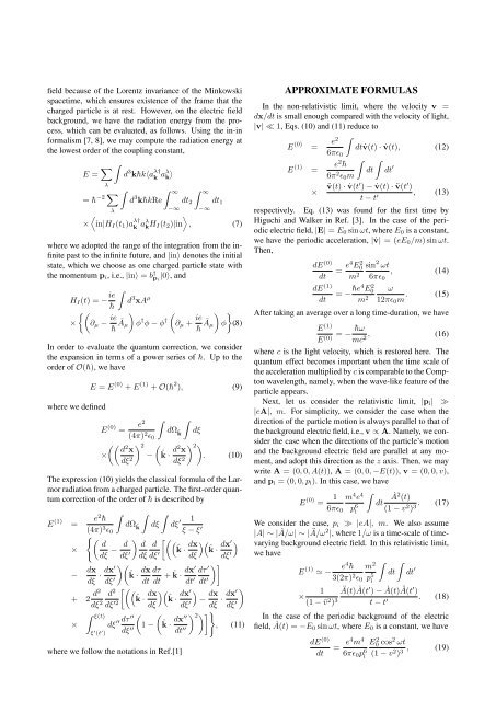
field because <str<strong>on</strong>g>of</str<strong>on</strong>g> the Lorentz <strong>in</strong>variance <str<strong>on</strong>g>of</str<strong>on</strong>g> the M<strong>in</strong>kowski<br />
spacetime, which ensures existence <str<strong>on</strong>g>of</str<strong>on</strong>g> the frame that the<br />
charged particle is at rest. However, <strong>on</strong> the electric field<br />
background, we have the radiati<strong>on</strong> energy from the process,<br />
which can be evaluated, as follows. Us<strong>in</strong>g the <strong>in</strong>-<strong>in</strong><br />
formalism [7, 8], we may compute the radiati<strong>on</strong> energy at<br />
the lowest order <str<strong>on</strong>g>of</str<strong>on</strong>g> the coupl<strong>in</strong>g c<strong>on</strong>stant,<br />
E = ∑<br />
∫<br />
λ<br />
∑<br />
∫<br />
−2<br />
= ¯h<br />
λ<br />
d 3 k¯hk〈a λ†<br />
k aλ k〉<br />
d 3 ∫ ∞ ∫ ∞<br />
k¯hkRe dt2<br />
−∞<br />
<br />
× <strong>in</strong>|HI(t1)a λ†<br />
k aλkHI(t2)|<strong>in</strong> dt1<br />
−∞<br />
<br />
, (7)<br />
where we adopted the range <str<strong>on</strong>g>of</str<strong>on</strong>g> the <strong>in</strong>tegrati<strong>on</strong> from the <strong>in</strong>f<strong>in</strong>ite<br />
past to the <strong>in</strong>f<strong>in</strong>ite future, and |<strong>in</strong>〉 denotes the <strong>in</strong>itial<br />
state, which we choose as <strong>on</strong>e charged particle state with<br />
the momentum pi, i.e., |<strong>in</strong>〉 = b † pi |0〉, and<br />
HI(t) = − ie<br />
∫<br />
d<br />
¯h<br />
3 xA µ<br />
{(<br />
× ∂µ − ie<br />
¯h Āµ<br />
)<br />
φ † φ − φ †<br />
(<br />
∂µ + ie<br />
¯h Āµ<br />
) }<br />
φ .(8)<br />
In order to evaluate the quantum correcti<strong>on</strong>, we c<strong>on</strong>sider<br />
the expansi<strong>on</strong> <strong>in</strong> terms <str<strong>on</strong>g>of</str<strong>on</strong>g> a power series <str<strong>on</strong>g>of</str<strong>on</strong>g> ¯h. Up to the<br />
order <str<strong>on</strong>g>of</str<strong>on</strong>g> O(¯h), we have<br />
where we def<strong>in</strong>ed<br />
E = E (0) + E (1) + O(¯h 2 ), (9)<br />
E (0) =<br />
(( 2 d x<br />
×<br />
dξ2 e2<br />
(4π) 2ɛ0 )2<br />
∫ ∫<br />
dΩˆ k dξ<br />
(<br />
− ˆk · d2x dξ2 )2)<br />
. (10)<br />
The expressi<strong>on</strong> (10) yields the classical formula <str<strong>on</strong>g>of</str<strong>on</strong>g> the Larmor<br />
radiati<strong>on</strong> from a charged particle. The first-order quantum<br />
correcti<strong>on</strong> <str<strong>on</strong>g>of</str<strong>on</strong>g> the order <str<strong>on</strong>g>of</str<strong>on</strong>g> ¯h is described by<br />
E (1) =<br />
e2¯h (4π) 3 ∫ ∫ ∫<br />
dΩˆ k dξ dξ<br />
ɛ0<br />
′ 1<br />
ξ − ξ ′<br />
×<br />
{ (<br />
d d<br />
−<br />
dξ dξ ′<br />
)<br />
d d<br />
dξ dξ ′<br />
[( (ˆk<br />
dx<br />
)(<br />
· ˆk<br />
dx<br />
·<br />
dξ<br />
′<br />
dξ ′<br />
)<br />
− dx dx′<br />
·<br />
dξ dξ ′<br />
)(<br />
ˆk · dx dτ<br />
dt dt + ˆ k · dx′<br />
dt ′<br />
dτ ′<br />
dt ′<br />
+<br />
)]<br />
2 d2<br />
dξ2 d2 dξ ′2<br />
[( (ˆk<br />
dx<br />
)(<br />
· ˆk<br />
dx<br />
·<br />
dξ<br />
′<br />
dξ ′<br />
)<br />
− dx dx′<br />
·<br />
dξ dξ ′<br />
×<br />
)<br />
∫ ξ(t) ′′<br />
′′ dτ<br />
dξ<br />
dξ ′′<br />
( (<br />
1 − ˆk · dx′′<br />
dt ′′<br />
) 2)] }<br />
, (11)<br />
ξ ′ (t ′ )<br />
where we follow the notati<strong>on</strong>s <strong>in</strong> Ref.[1]<br />
APPROXIMATE FORMULAS<br />
In the n<strong>on</strong>-relativistic limit, where the velocity v =<br />
dx/dt is small enough compared with the velocity <str<strong>on</strong>g>of</str<strong>on</strong>g> light,<br />
|v| ≪ 1, Eqs. (10) and (11) reduce to<br />
E (0) e<br />
=<br />
2 ∫<br />
dt ˙v(t) · ˙v(t), (12)<br />
6πɛ0<br />
E (1) =<br />
e 2 ¯h<br />
6π 2 ɛ0m<br />
∫ ∫<br />
dt dt ′<br />
× ¨v(t) · ˙v(t′ ) − ˙v(t) · ¨v(t ′ )<br />
t − t ′ , (13)<br />
respectively. Eq. (13) was found for the first time by<br />
Higuchi and Walker <strong>in</strong> Ref. [3]. In the case <str<strong>on</strong>g>of</str<strong>on</strong>g> the periodic<br />
electric field, |E| = E0 s<strong>in</strong> ωt, where E0 is a c<strong>on</strong>stant,<br />
we have the periodic accelerati<strong>on</strong>, | ˙v| = (eE0/m) s<strong>in</strong> ωt.<br />
Then,<br />
dE (0)<br />
dt = e4E2 0<br />
m2 dE (1)<br />
dt = −¯he4 E2 0<br />
m2 s<strong>in</strong> 2 ωt<br />
,<br />
6πɛ0<br />
(14)<br />
ω<br />
.<br />
12πɛ0m<br />
(15)<br />
After tak<strong>in</strong>g an average over a l<strong>on</strong>g time-durati<strong>on</strong>, we have<br />
E (1)<br />
E<br />
¯hω<br />
= − , (16)<br />
(0) mc2 where c is the light velocity, which is restored here. The<br />
quantum effect becomes important when the time scale <str<strong>on</strong>g>of</str<strong>on</strong>g><br />
the accelerati<strong>on</strong> multiplied by c is comparable to the Compt<strong>on</strong><br />
wavelength, namely, when the wave-like feature <str<strong>on</strong>g>of</str<strong>on</strong>g> the<br />
particle appears.<br />
Next, let us c<strong>on</strong>sider the relativistic limit, |pi| ≫<br />
|eA|, m. For simplicity, we c<strong>on</strong>sider the case when the<br />
directi<strong>on</strong> <str<strong>on</strong>g>of</str<strong>on</strong>g> the particle moti<strong>on</strong> is always parallel to that <str<strong>on</strong>g>of</str<strong>on</strong>g><br />
the background electric field, i.e., v ∝ A. Namely, we c<strong>on</strong>sider<br />
the case when the directi<strong>on</strong>s <str<strong>on</strong>g>of</str<strong>on</strong>g> the particle’s moti<strong>on</strong><br />
and the background electric field are parallel at any moment,<br />
and adopt this directi<strong>on</strong> as the z axis. Then, we may<br />
write A = (0, 0, A(t)), A ˙ = (0, 0, −E(t)), v = (0, 0, v),<br />
and pi = (0, 0, pi). In this case, we have<br />
E (0) = 1 m<br />
6πɛ0<br />
4e4 p6 i<br />
∫<br />
dt<br />
˙<br />
A 2 (t)<br />
(1 − v2 . (17)<br />
) 3<br />
We c<strong>on</strong>sider the case, pi ≫ |eA|, m. We also assume<br />
|A| ∼ | ˙ A/ω| ∼ | Ä/ω2 |, where 1/ω is a time-scale <str<strong>on</strong>g>of</str<strong>on</strong>g> timevary<strong>in</strong>g<br />
background electric field. In this relativistic limit,<br />
we have<br />
E (1) − e4¯h 3(2π) 2 m<br />
ɛ0<br />
2<br />
p5 ∫ ∫<br />
dt dt<br />
i<br />
′<br />
×<br />
1<br />
(1 − ¯v 2 ) 3<br />
Ä(t) ˙ A(t ′ ) − ˙ A(t) Ä(t′ )<br />
t − t ′ . (18)<br />
In the case <str<strong>on</strong>g>of</str<strong>on</strong>g> the periodic background <str<strong>on</strong>g>of</str<strong>on</strong>g> the electric<br />
field, ˙<br />
A(t) = −E0 s<strong>in</strong> ωt, where E0 is a c<strong>on</strong>stant, we have<br />
dE (0)<br />
dt = e4 m 4<br />
6πɛ0p 6 i<br />
E2 0 cos2 ωt<br />
(1 − v2 , (19)<br />
) 3