Proceedings of International Conference on Physics in ... - KEK
Proceedings of International Conference on Physics in ... - KEK
Proceedings of International Conference on Physics in ... - KEK

Create successful ePaper yourself
Turn your PDF publications into a flip-book with our unique Google optimized e-Paper software.
under the assumpti<strong>on</strong> <str<strong>on</strong>g>of</str<strong>on</strong>g> the symmetry al<strong>on</strong>g it. gtt, gxx<br />
and gzz are the <strong>in</strong>duced world-volume metric, and they are<br />
equal to the background metric (1) except for gzz = 1/z 2 +<br />
θ ′ (z) 2 .<br />
NONLINEAR CONDUCTIVITY<br />
It was found [6] that the <strong>on</strong>-shell D7-brane acti<strong>on</strong> becomes<br />
complex unless we choose a specific comb<strong>in</strong>ati<strong>on</strong> <str<strong>on</strong>g>of</str<strong>on</strong>g><br />
J and E; the relati<strong>on</strong>ship between J and E is determ<strong>in</strong>ed<br />
by the reality c<strong>on</strong>diti<strong>on</strong> <str<strong>on</strong>g>of</str<strong>on</strong>g> the <strong>on</strong>-shell acti<strong>on</strong>, hence, J is<br />
obta<strong>in</strong>ed as a n<strong>on</strong>l<strong>in</strong>ear functi<strong>on</strong> <str<strong>on</strong>g>of</str<strong>on</strong>g> E. The <strong>on</strong>-shell acti<strong>on</strong><br />
is given by [6] ¯ SD7 = −N ∫ dzdtd 3 x √ ¯gzz|gtt| −1√ F1F2<br />
with F1 = |gtt|gxx − E 2 and F2 = |gtt|g 2 xx cos 6 ¯ θ −<br />
gxxJ 2 /N 2 , where ¯gzz is the <strong>in</strong>duced metric given by ¯ θ,<br />
which is the <strong>on</strong>-shell c<strong>on</strong>figurati<strong>on</strong> <str<strong>on</strong>g>of</str<strong>on</strong>g> θ(z). S<strong>in</strong>ce both F1<br />
and F2 cross zero somewhere between the boundary and<br />
the horiz<strong>on</strong>, the <strong>on</strong>ly way to make ¯ SD7 real is to choose<br />
J and E so that F1 and F2 cross zero at the same po<strong>in</strong>t<br />
z = z∗. The hypersurface given by z = z∗ is <str<strong>on</strong>g>of</str<strong>on</strong>g>ten<br />
called the “s<strong>in</strong>gular shell”. Then, the reality c<strong>on</strong>diti<strong>on</strong><br />
F1(z∗) = F2(z∗) = 0 gives us the relati<strong>on</strong>ship between<br />
J and E <strong>in</strong> the form <str<strong>on</strong>g>of</str<strong>on</strong>g> J = σ0E [6], where<br />
σ0 = N T (e 2 + 1) 1/4 cos 3 ¯ θ(z∗). (3)<br />
Our task is to solve the equati<strong>on</strong> <str<strong>on</strong>g>of</str<strong>on</strong>g> moti<strong>on</strong> (EOM) for θ<br />
to obta<strong>in</strong> the explicit representati<strong>on</strong>. ¯ θ(z) can be expanded<br />
as ¯ θ(z) = mqz + O(z 3 ), where mq is the current quark<br />
mass [13], which is a parameter <str<strong>on</strong>g>of</str<strong>on</strong>g> the microscopic theory.<br />
mq is related to the gap <strong>in</strong> c<strong>on</strong>densed matters.<br />
Let us choose the temperature to be T = √ 2/π so that<br />
zH = 1, e = E/2 and z∗ = √ E 2 /4 + 1 − E/2. 4 We<br />
further fix NcNf = 40. NcNf governs the pair-creati<strong>on</strong><br />
rate <str<strong>on</strong>g>of</str<strong>on</strong>g> the charge carriers as we shall expla<strong>in</strong> later. We<br />
need to solve the EOM for θ numerically. The boundary<br />
c<strong>on</strong>diti<strong>on</strong> we employ is θ(z)/z|z=0 = mq and we request<br />
the absence <str<strong>on</strong>g>of</str<strong>on</strong>g> s<strong>in</strong>gularity <strong>in</strong> the D7-brane c<strong>on</strong>figurati<strong>on</strong>.<br />
For earlier studies <strong>on</strong> the n<strong>on</strong>l<strong>in</strong>ear c<strong>on</strong>ductivity by us<strong>in</strong>g<br />
this method, see for example, Refs. [7, 8].<br />
RESULTS<br />
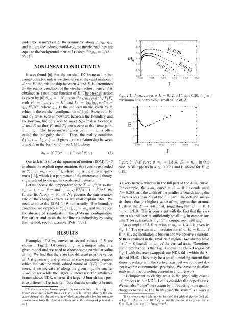
Examples <str<strong>on</strong>g>of</str<strong>on</strong>g> J-mq curves at several values <str<strong>on</strong>g>of</str<strong>on</strong>g> E are<br />
shown <strong>in</strong> Fig. 2. Of course, mq has a unique value at a<br />
given model and we need to choose some particular value<br />
<str<strong>on</strong>g>of</str<strong>on</strong>g> mq. We f<strong>in</strong>d that there are two different possible values<br />
<str<strong>on</strong>g>of</str<strong>on</strong>g> J at given mq and given E <strong>in</strong> some parameter regi<strong>on</strong>,<br />
which <strong>in</strong>dicate the multi-valued nature <str<strong>on</strong>g>of</str<strong>on</strong>g> J(E). Furthermore,<br />
if we <strong>in</strong>crease E al<strong>on</strong>g the given mq, the smaller<br />
J decreases while the larger J <strong>in</strong>creases; the smaller-J<br />
branch shows NDR, whereas the larger-J branch has a positive<br />
differential resistivity. Note that the smaller-J branch<br />
4 In this article, we have employed the natural units c = ¯h = kB = 1.<br />
If our scale unit is meV (mili eV), T ∼ 5 K. If we identify the unit<br />
quark charge with the unit charge <str<strong>on</strong>g>of</str<strong>on</strong>g> electr<strong>on</strong>s, the effective f<strong>in</strong>e-structure<br />
c<strong>on</strong>stant read from the Coulomb <strong>in</strong>teracti<strong>on</strong> <strong>in</strong> the <strong>in</strong>ter-quark potential is<br />
∼ 1.<br />
mq<br />
1.34<br />
1.33<br />
1.32<br />
1.31<br />
1.30<br />
1.29<br />
E0.12<br />
E0.20<br />
E0.15<br />
1.28<br />
0.000 0.005 0.010 0.015 0.020 0.025<br />
Figure 2: J-mq curves at E = 0.12, 0.15, and 0.20. mq is<br />
maximum at a n<strong>on</strong>zero but small value <str<strong>on</strong>g>of</str<strong>on</strong>g> J.<br />
E<br />
0.25<br />
0.20<br />
0.15<br />
0.10<br />
0.05<br />
0.00<br />
0.000 0.005 0.010 0.015 0.020 0.025<br />
Figure 3: J-E curve at mq = 1.315. Ec = 0.11 <strong>in</strong> this<br />
case. NDR appears <strong>in</strong> J ≤ 0.0031 and is absent for E ≥<br />
0.19.<br />
is a very narrow w<strong>in</strong>dow <strong>in</strong> the full part <str<strong>on</strong>g>of</str<strong>on</strong>g> the J-mq curve.<br />
For example, the J-mq curve at E = 0.2 extends until<br />
J = 0.288, and the width <str<strong>on</strong>g>of</str<strong>on</strong>g> the smaller-J branch al<strong>on</strong>g the<br />
J axes is less than 2% <str<strong>on</strong>g>of</str<strong>on</strong>g> the full part. The detailed analysis<br />
shows that the highest value <str<strong>on</strong>g>of</str<strong>on</strong>g> mq approaches around<br />
1.310 at the E → +0 limit, suggest<strong>in</strong>g that Ec = 0 if<br />
mq < 1.310. This is c<strong>on</strong>sistent with the fact that the system<br />
is a c<strong>on</strong>ductor at sufficiently small mq <strong>in</strong> comparis<strong>on</strong><br />
with T (or sufficiently high T <strong>in</strong> comparis<strong>on</strong> with mq).<br />
An example <str<strong>on</strong>g>of</str<strong>on</strong>g> J-E relati<strong>on</strong> at mq = 1.315 is given <strong>in</strong><br />
Fig. 3. 5 The system is an <strong>in</strong>sulator for E < Ec = 0.11. If<br />
E ≥ Ec, the <strong>in</strong>sulati<strong>on</strong> is broken and we observe a current.<br />
NDR is realized <strong>in</strong> the smaller-J regi<strong>on</strong>. We always have<br />
the J = 0 branch <strong>on</strong> top <str<strong>on</strong>g>of</str<strong>on</strong>g> the vertical axis. Therefore,<br />
our <strong>in</strong>terpretati<strong>on</strong> is that Fig. 3 shows the B-C-D regi<strong>on</strong> <str<strong>on</strong>g>of</str<strong>on</strong>g><br />
Fig. 1 with the axes swapped; our NDR falls with<strong>in</strong> the Sshaped<br />
NDR. There may be a small tunnel<strong>in</strong>g current that<br />
almost overlaps with the vertical axis, but we could not detect<br />
it with<strong>in</strong> our numerical precisi<strong>on</strong>. We leave the detailed<br />
analysis <strong>on</strong> the tunnel<strong>in</strong>g current <strong>in</strong> a future work.<br />
It is important to clarify what is the physically essential<br />
process <strong>in</strong> our NDR. Let us c<strong>on</strong>sider the doped cases.<br />
We can also “dope” the system by <strong>in</strong>troduc<strong>in</strong>g f<strong>in</strong>ite quarkcharge<br />
density [14, 15]. In this case, the system is always a<br />
5 If we choose our scale unit to be meV, the critical electric field Ec<br />
<strong>in</strong> Fig. 3 is Ec ∼ 5 × 10 −1 V/m, and the current density realized at<br />
E = Ec is J ∼ 1 × 10 −4 mA/mm 2 .<br />
J<br />
J