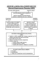
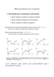
Untitled - Cdm.unimo.it

234 Polynomial Approximation of Differential Equations
Once the stability of the scheme is achieved, error estimates are obtained by applying
the same proof to the error pn − Un, where Un ∈ Pn, n ≥ 1 , is a suitable projection
of U. The same argument was used in section 10.2 for the heat equation (see also
canuto, hussaini, quarteroni and zang(1988), chapter 10). Other spectral type
approximations and theoretical results relative to equation (10.3.1) are considered in
gottlieb and orszag(1977), section 8, gottlieb(1981), canuto and quarteroni
(1982b), mercier(1982), mercier(1989), tal-ezer(1986b), dubiner(1987).
Similar results are available for the equation
(10.3.20)
∂U ∂U
(x,t) = ζ (x,t), ∀x ∈ [−1,1[, ∀t ∈]0,T],
∂t ∂x
when the boundary condition is imposed at the point x = 1.
The reader should pay a little more care to the theoretical analysis of partial differ-
ential equations, before trying experiments on general problems, such as the following
one:
(10.3.21)
∂U
(x,t) = A(x,U(x,t))∂U (x,t), x ∈] − 1,1[, t ∈]0,T],
∂t ∂x
where A :] − 1,1[×R → R is given.
An analysis for equations such as (10.3.21) is carried out in smoller(1983), rhee,
aris and amundson(1986), kreiss and lorenz(1989). It is known that the solution
of (10.3.21) maintains a constant value along the so-called characteristic curves. These
are parallel straight-lines in the (x,t) plane with slope 1/ζ for equation (10.3.1), and
slope −1/ζ for equation (10.3.20). In the former case, the solution U(x, ·), x ∈ [−1,1],
shifts on the right-hand side during the time evolution. With terminology deriving from
fluid physics, the point x = −1 is the inflow boundary, while x = 1 is the outflow
boundary. The situation is reversed for equation (10.3.20). The characteristic curves
are no longer straight-lines when A is not a constant. Even in the case of smooth initial
conditions and smooth boundary data, the solution can loose regularity and shocks can
be generated when two or more characteristic curves intersect. The numerical analysis
becomes a delicate issue in this situation, especially for spectral methods which are