Untitled - Cdm.unimo.it

Time-Dependent Problems 245
It is well-known that, when condition (10.6.4) is violated, severe instabilities can
occur when applying the algorithm (10.6.2). Actually, (10.6.4) is equivalent to requiring
that the spectral radius ρ(I + hD) is less than 1 (see section 7.6). This stresses the
importance of working with matrices having eigenvalues with a negative real part. All
the examples analyzed in the previous sections lead to systems of ordinary differential
equations where the corresponding matrices fulfill such a requirement (see chapter eight).
Moreover, in some cases (see (10.3.8), (10.3.19) and (10.5.11)), we were able to prove an
additional property, that is, that a certain norm in R n of the vector ¯p(t) is a decreasing
function of t ∈ [0,T]. This automatically excludes the existence of eigenvalues with a
positive real part, otherwise the components of the vector ¯p along the directions of
the corresponding eigenvectors would be amplified during the time evolution. Due to
(10.6.3), the error committed at time T decays linearly with the size of the interval h.
This means that the method is first-order accurate. We observe that the constant C in
(10.6.3) depends on n.
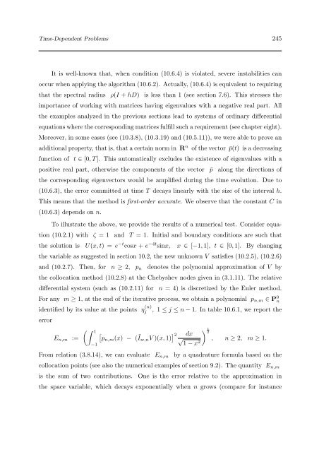
To illustrate the above, we provide the results of a numerical test. Consider equa-
tion (10.2.1) with ζ = 1 and T = 1. Initial and boundary conditions are such that
the solution is U(x,t) = e −t cosx + e −4t sinx, x ∈ [−1,1], t ∈ [0,1]. By changing
the variable as suggested in section 10.2, the new unknown V satisfies (10.2.5), (10.2.6)
and (10.2.7). Then, for n ≥ 2, pn denotes the polynomial approximation of V by
the collocation method (10.2.8) at the Chebyshev nodes given in (3.1.11). The relative
differential system (such as (10.2.11) for n = 4) is discretized by the Euler method.
For any m ≥ 1, at the end of the iterative process, we obtain a polynomial pn,m ∈ P 0 n
identified by its value at the points η (n)
j , 1 ≤ j ≤ n − 1. In table 10.6.1, we report the
error
En,m :=
1
−1
pn,m(x) − ( Ĩw,nV )(x,1)
2 dx
√
1 − x2 1
2
, n ≥ 2, m ≥ 1.
From relation (3.8.14), we can evaluate En,m by a quadrature formula based on the
collocation points (see also the numerical examples of section 9.2). The quantity En,m
is the sum of two contributions. One is the error relative to the approximation in
the space variable, which decays exponentially when n grows (compare for instance