Untitled - Cdm.unimo.it

254 Polynomial Approximation of Differential Equations
Thus, our collocation scheme is now in a variational form. On the other hand, U satisfies
I U ′ ψ ′ dx =
I fψdx, ∀ψ ∈ X, ψ(s0) = ψ(sm) = 0, where X is the Hilbert space
with norm ψX =
I ψ2dx +
I [ψ′ ] 2dx 1/2 . Due to theorem 9.4.1, it is sufficient to
estimate the quantity
I fφdx − Fn(φ) , ∀φ ∈ Xn, to conclude that the error |U −πn|
tends to zero in the norm of X. To this end, for any Sk, we can argue as in (9.4.12),
(9.4.13), which lead to (11.2.9).
With some technical modifications, we can use the same proof to obtain a conver-
gence result for the scheme (11.2.4), (11.2.5), (11.2.6), (11.2.7), in the Legendre case.
For other sets of collocation nodes the theory becomes more difficult. The idea is to
recast the collocation scheme into a variational framework which then reduces to a
problem like (9.4.16) in each subdomain.
We get similar conclusions when different degrees nk, 1 ≤ k ≤ m, are assigned to
the approximating polynomials. Now, we can either use condition (11.2.6) as is, or con-
dition (11.2.8) after suitable modification. For example, in the Legendre case, starting
from the variational formulation (11.2.11), we deduce that the following relations are
satisfied at the interface nodes:
(11.2.12) − ˜w (nk,k)
nk
+ γk
where γk := 1 ( ˜w (nk,k)
nk
+ ˜w (nk+1,k+1)
−1
0
˜w (nk,k)
nk
p ′′ nk,k + ˜w (nk+1,k+1)
0 p ′′
nk+1,k+1 (sk)
p ′ nk,k − p ′
nk+1,k+1 (sk) = f(sk) 1 ≤ k ≤ m − 1,
+ ˜w (nk+1,k+1)
0 ), 1 ≤ k ≤ m − 1.
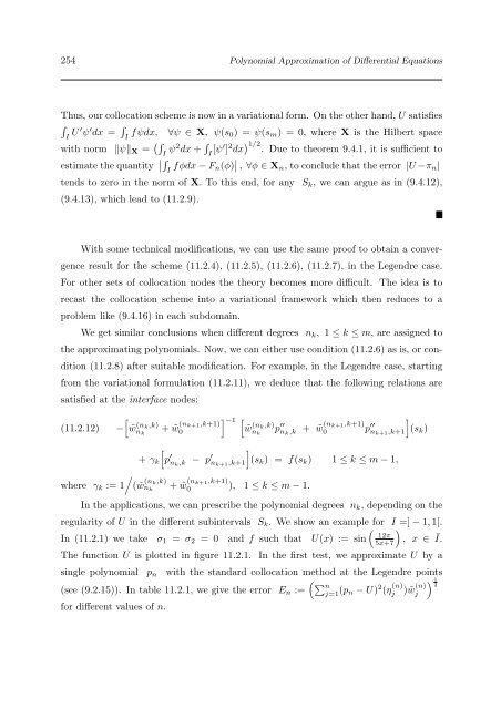
In the applications, we can prescribe the polynomial degrees nk, depending on the
regularity of U in the different subintervals Sk. We show an example for I =] − 1,1[.
In (11.2.1) we take σ1 = σ2 = 0 and f such that U(x) := sin
12π
5x+7
, x ∈ Ī.
The function U is plotted in figure 11.2.1. In the first test, we approximate U by a
single polynomial pn with the standard collocation method at the Legendre points
(see (9.2.15)). In table 11.2.1, we give the error En :=
for different values of n.
n j=1 (pn − U) 2 (η (n)
j ) ˜w (n)
j
1
2