Polymers in Confined Geometry.pdf

2.3. SEMI-FLEXIBLE POLYMERS 13
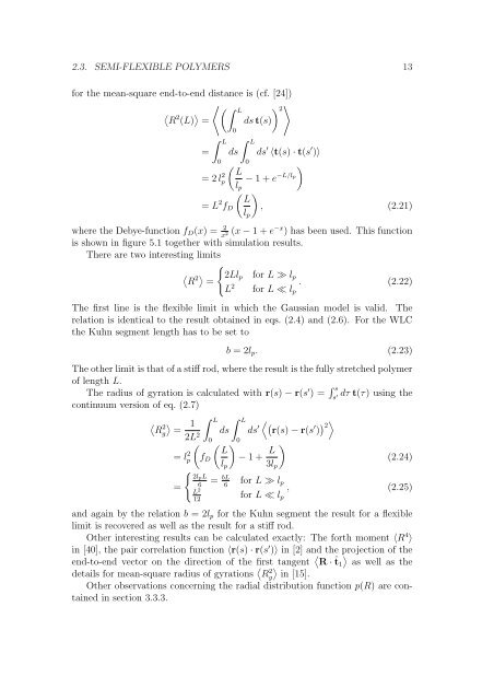
for the mean-square end-to-end distance is (cf. [24])
L
2
2
R (L) = ds t(s)
L
0
L
ds
0
′ 〈t(s) · t(s ′ )〉
= ds
0
= 2 l 2
L
p − 1 + e
lp
−L/lp
= L 2
L
fD , (2.21)
where the Debye-function fD(x) = 2
x2 (x − 1 + e−x ) has been used. This function
is shown in figure 5.1 together with simulation results.
There are two interesting limits
2
R
2Llp for L ≫ lp
=
L2 . (2.22)
for L ≪ lp
The first line is the flexible limit in which the Gaussian model is valid. The
relation is identical to the result obtained in eqs. (2.4) and (2.6). For the WLC
the Kuhn segment length has to be set to
lp
b = 2lp. (2.23)
The other limit is that of a stiff rod, where the result is the fully stretched polymer
of length L.
The radius of gyration is calculated with r(s) − r(s ′ ) = s
s ′ dτ t(τ) using the
continuum version of eq. (2.7)
2 1
Rg =
2L2 = l 2
p
=
L
0
fD
2lpL
6
L2 12
L
ds ′
r(s)
′ 2
− r(s )
ds
0
L
− 1 + L
lp
= bL
6
3lp
(2.24)
for L ≫ lp
, (2.25)
for L ≪ lp
and again by the relation b = 2lp for the Kuhn segment the result for a flexible
limit is recovered as well as the result for a stiff rod.
Other interesting results can be calculated exactly: The forth moment 〈R4 〉
in [40], the pair correlation function 〈r(s) · r(s ′ )〉 in [2] and the projection of the
end-to-end vector on the direction of the first tangent
R · ˆt1 as well as the
details for mean-square radius of gyrations R2
g in [15].
Other observations concerning the radial distribution function p(R) are contained
in section 3.3.3.