Polymers in Confined Geometry.pdf

5.2. THE HARMONIC POTENTIAL 59
ˆt(0.5) · ˆt(s + 0.5)
1
0.1
0.01
0.001
-0.5
-0.4
-0.3
-0.2
exact
simulation
-0.1 0
s − 0.5
0.1
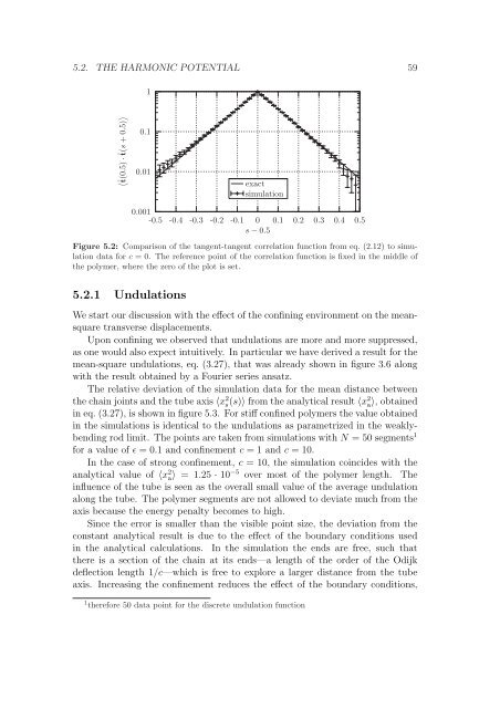
Figure 5.2: Comparison of the tangent-tangent correlation function from eq. (2.12) to simulation
data for c = 0. The reference point of the correlation function is fixed in the middle of
the polymer, where the zero of the plot is set.
5.2.1 Undulations
We start our discussion with the effect of the confining environment on the meansquare
transverse displacements.
Upon confining we observed that undulations are more and more suppressed,
as one would also expect intuitively. In particular we have derived a result for the
mean-square undulations, eq. (3.27), that was already shown in figure 3.6 along
with the result obtained by a Fourier series ansatz.
The relative deviation of the simulation data for the mean distance between
the chain joints and the tube axis 〈x 2 s(s)〉 from the analytical result 〈x 2 a〉, obtained
in eq. (3.27), is shown in figure 5.3. For stiff confined polymers the value obtained
in the simulations is identical to the undulations as parametrized in the weaklybending
rod limit. The points are taken from simulations with N = 50 segments 1
for a value of ɛ = 0.1 and confinement c = 1 and c = 10.
In the case of strong confinement, c = 10, the simulation coincides with the
analytical value of 〈x 2 a〉 = 1.25 · 10 −5 over most of the polymer length. The
influence of the tube is seen as the overall small value of the average undulation
along the tube. The polymer segments are not allowed to deviate much from the
axis because the energy penalty becomes to high.
Since the error is smaller than the visible point size, the deviation from the
constant analytical result is due to the effect of the boundary conditions used
in the analytical calculations. In the simulation the ends are free, such that
there is a section of the chain at its ends—a length of the order of the Odijk
deflection length 1/c—which is free to explore a larger distance from the tube
axis. Increasing the confinement reduces the effect of the boundary conditions,
1 therefore 50 data point for the discrete undulation function
0.2
0.3
0.4
0.5