Polymers in Confined Geometry.pdf

32 CHAPTER 3. POLYMERS IN CONFINED GEOMETRY
R 2 (L) /L 2
1
0.9
0.8
0.7
0.6
0.5
0.4
0.3
0.01
0.1
1
L/ld
10
lp/L = 0.1
lp/L = 0.5
lp/L = 1
lp/L = 5
lp/L = 10
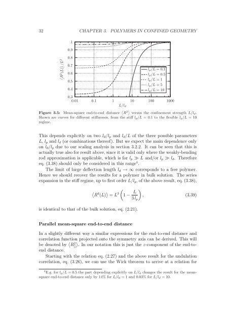
Figure 3.5: Mean-square end-to-end distance R 2 versus the confinement strength L/ld.
Shown are curves for different stiffnesses, from the stiff lp/L = 0.1 to the flexible lp/L = 10
regime.
This depends explicitly on two ld/lp and ld/L of the three possible parameters
L, lp and ld (or combinations thereof). But we expect the main dependence only
on ld/lp due to our scaling analysis in section 3.2.2. It can be seen that this is
actually true also for result above, since it is valid only where the weakly-bending
rod approximation is applicable, which is for lp ≫ L and/or lp ≫ ld. Therefore
eq. (3.38) should only be considered in this range 4 .
The limit of large deflection length ld → ∞ corresponds to a free polymer.
Hence we should recover the results for a polymer in bulk solution. The series
expansion in the stiff regime, up to first order L/lp, of the above result, eq. (3.38),
is identical to that of the bulk solution, eq. (2.21).
Parallel mean-square end-to-end distance
100
1000
2 2
R (L) = L 1 − L
, (3.39)
3 lp
In a slightly different way a similar expressions for the end-to-end distance and
correlation function projected onto the symmetry axis can be derived. This will
be denoted by R2
|| . In our notation this is just the z-component of the end-toend
distance.
Starting with the relation eq. (2.27) and the above result for the undulation
correlation, eq. (3.26), we can use the Wick theorem to arrive at a relation for
4 E.g. for lp/L = 0.5 the part depending explicitly on L/ld changes the result for the meansquare
end-to-end distance only by 14% for L/ld = 1 and 0.03% for L/ld = 10.