Polymers in Confined Geometry.pdf

5.2. THE HARMONIC POTENTIAL 61
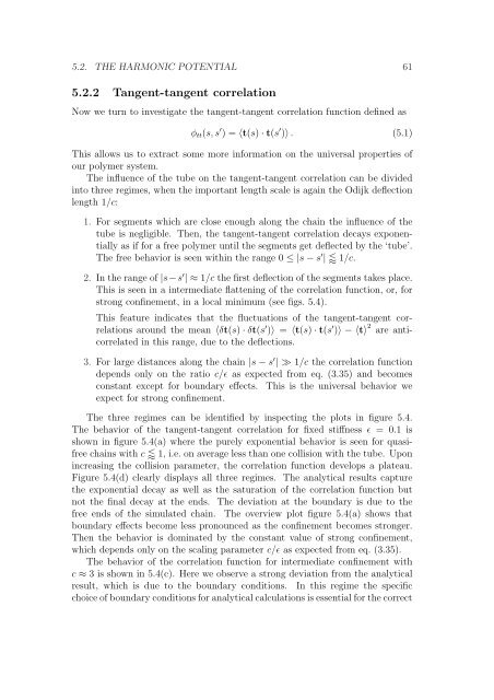
5.2.2 Tangent-tangent correlation
Now we turn to investigate the tangent-tangent correlation function defined as
φtt(s, s ′ ) = 〈t(s) · t(s ′ )〉 . (5.1)
This allows us to extract some more information on the universal properties of
our polymer system.
The influence of the tube on the tangent-tangent correlation can be divided
into three regimes, when the important length scale is again the Odijk deflection
length 1/c:
1. For segments which are close enough along the chain the influence of the
tube is negligible. Then, the tangent-tangent correlation decays exponentially
as if for a free polymer until the segments get deflected by the ‘tube’.
The free behavior is seen within the range 0 ≤ |s − s ′ | 1/c.
2. In the range of |s−s ′ | ≈ 1/c the first deflection of the segments takes place.
This is seen in a intermediate flattening of the correlation function, or, for
strong confinement, in a local minimum (see figs. 5.4).
This feature indicates that the fluctuations of the tangent-tangent correlations
around the mean 〈δt(s) · δt(s ′ )〉 = 〈t(s) · t(s ′ )〉 − 〈t〉 2 are anticorrelated
in this range, due to the deflections.
3. For large distances along the chain |s − s ′ | ≫ 1/c the correlation function
depends only on the ratio c/ɛ as expected from eq. (3.35) and becomes
constant except for boundary effects. This is the universal behavior we
expect for strong confinement.
The three regimes can be identified by inspecting the plots in figure 5.4.
The behavior of the tangent-tangent correlation for fixed stiffness ɛ = 0.1 is
shown in figure 5.4(a) where the purely exponential behavior is seen for quasifree
chains with c 1, i.e. on average less than one collision with the tube. Upon
increasing the collision parameter, the correlation function develops a plateau.
Figure 5.4(d) clearly displays all three regimes. The analytical results capture
the exponential decay as well as the saturation of the correlation function but
not the final decay at the ends. The deviation at the boundary is due to the
free ends of the simulated chain. The overview plot figure 5.4(a) shows that
boundary effects become less pronounced as the confinement becomes stronger.
Then the behavior is dominated by the constant value of strong confinement,
which depends only on the scaling parameter c/ɛ as expected from eq. (3.35).
The behavior of the correlation function for intermediate confinement with
c ≈ 3 is shown in 5.4(c). Here we observe a strong deviation from the analytical
result, which is due to the boundary conditions. In this regime the specific
choice of boundary conditions for analytical calculations is essential for the correct