Polymers in Confined Geometry.pdf

68 CHAPTER 5. SIMULATION RESULTS
〈Ra〉
1
0.8
0.6
0.4
0.2
0
0.1
1
10
c/ɛ
experimental data
Odijk scaling (fit)
ɛ = 0.1
ɛ = 0.5
ɛ = 1
ɛ = 5
ɛ = 10
ɛ = 50
ɛ = 300
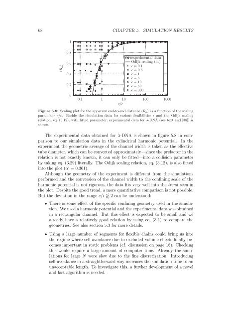
Figure 5.8: Scaling plot for the apparent end-to-end distance 〈Ra〉 as a function of the scaling
parameter c/ɛ. Beside the simulation data for various flexibilities ɛ and the Odijk scaling
relation, eq. (3.12), with fitted parameter, experimental data for λ-DNA (see text and [38]) is
shown.
The experimental data obtained for λ-DNA is shown in figure 5.8 in comparison
to our simulation data in the cylindrical harmonic potential. In the
experiment the geometric average of the channel width is taken as the effective
tube diameter, which can be converted approximately—since the prefactor in the
relation is not exactly known, it can only be fitted—into a collision parameter
by taking eq. (3.29) literally. The Odijk scaling relation, eq. (3.12), is also fitted
into the plot (α ′ = 0.361).
Although the geometry of the experiment is different from the simulations
performed and the conversion of the channel width to the confining scale of the
harmonic potential is not rigorous, the data fits very well into the trend seen in
the plot. Despite the good trend, a more quantitative comparison is not possible.
But the deviation in the range c/ɛ 2 can be understood:
100
1000
• There is some effect of the specific confining geometry used in the simulation.
We used a harmonic potential and the experimental data was obtained
in a rectangular channel. But this effect is expected to be small and we
already have a relatively good relation by using eq. (3.1) to compare the
geometries. See also section 5.3 for more details.
• Using a large number of segments for flexible chains could bring us into
the regime where self-avoidance due to excluded volume effects finally becomes
important in static problems (cf. discussion on page 18). Checking
this would require a large amount of computer time. Already the simulations
for large N were slow due to the fine discretization. Introducing
self-avoidance in a straightforward way increases the simulation time to an
unacceptable length. To investigate this, a further development of a novel
and fast algorithm is needed.