Polymers in Confined Geometry.pdf

More documents

Recommendations

Info

64 CHAPTER 5. SIMULATION RESULTS Comparison of analytic and simulation results Even if one measures all length in units of the total polymer length L, the meansquare end-to-end distance is still a function of two length scales, the tube diameter d and the persistence length lp. As discussed in section 3.2 this suggests to introduce two dimensionless parameters, ɛ = L/lp as a measure of the polymer stiffness and c = L/ld counting the number of collision of the polymer with the tube and being related to the tube diameter through the relation in eq. (3.1). In the discussion we have to distinguish the limiting cases of stiff (ɛ ≪ 1) and flexible polymers (ɛ ≫ 1). In the stiff limit the main parameter characterizing the influence of the confinement on the polymer conformation is the collision parameter c. For c ≪ 1 the polymer is unconfined and behaves as a free polymer with 〈R 2 〉 ∼ L 2 (cf. eq. (2.22)). For c ≈ 1 undulations for the filament are not yet restricted but the overall rotation of the filament is hindered by the walls. For c ≫ 1 there is strong confinement with many collisions of the polymer with the wall. In the flexible limit the critical scales to compare are the radius of gyration Rg and the tube diameter. As noted by de Gennes the scaling behavior of the unconfined chain, 〈R 2 〉 ∼ lpL, starts to change once the mean-square end-to-end distance becomes comparable to the tube diameter d. Then the polymer starts to stretch due to the excluded volume interaction of distant segments along the chain, such that 〈R 2 〉 ∼ Lc/ɛ. Here we consider phantom chains where selfavoidance effects are neglected. Hence, as discussed in section 3.2.1 one expects no effect at all of confinement on the polymer configuration. A stretching for a chain consisting of segments is then only due to the finite segment length. Even for flexible chains stiffness effects will become important once the tube diameter becomes comparable with the persistence length. Then the same arguments as in the stiff case apply. From the foregoing discussion we can expect to find universal behavior for stiff chains, when the chain starts to be deflected, c 1. Since we expect to have a dependence on the scaling parameter c/ɛ this means c ɛ ɛ−1 . (5.2) On the other hand for flexible chains the relevant condition is that the tube diameter is of the order of the segment length or less d lp which leads through eq. (3.1) to c 1 (5.3) ɛ for the scaling parameter. We can summarize this conditions for the universal scaling regime in c max(1, ɛ ɛ univ −1 ). (5.4) For flexible polymers we therefore expect to have a longer scaling regime.
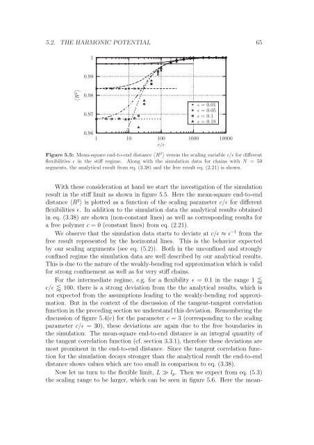
5.2. THE HARMONIC POTENTIAL 65 R 2 1 0.99 0.98 0.97 0.96 1 10 100 c/ɛ 1000 ɛ = 0.01 ɛ = 0.05 ɛ = 0.1 ɛ = 0.18 10000 Figure 5.5: Mean-square end-to-end distance R 2 versus the scaling variable c/ɛ for different flexibilities ɛ in the stiff regime. Along with the simulation data for chains with N = 50 segments, the analytical result from eq. (3.38) and the free result eq. (2.21) is shown. With these consideration at hand we start the investigation of the simulation result in the stiff limit as shown in figure 5.5. Here the mean-square end-to-end distance 〈R 2 〉 is plotted as a function of the scaling parameter c/ɛ for different flexibilities ɛ. In addition to the simulation data the analytical results obtained in eq. (3.38) are shown (non-constant lines) as well as corresponding results for a free polymer c = 0 (constant lines) from eq. (2.21). We observe that the simulation data starts to deviate at c/ɛ ≈ ɛ −1 from the free result represented by the horizontal lines. This is the behavior expected by our scaling arguments (see eq. (5.2)). Both in the unconfined and strongly confined regime the simulation data are well described by our analytical results. This is due to the nature of the weakly-bending rod approximation which is valid for strong confinement as well as for very stiff chains. For the intermediate regime, e.g. for a flexibility ɛ = 0.1 in the range 1 c/ɛ 100, there is a strong deviation from the the analytical results, which is not expected from the assumptions leading to the weakly-bending rod approximation. But in the context of the discussion of the tangent-tangent correlation function in the preceding section we understand this deviation. Remembering the discussion of figure 5.4(c) for the parameter c = 3 (corresponding to the scaling parameter c/ɛ = 30), these deviations are again due to the free boundaries in the simulation. The mean-square end-to-end distance is an integral quantity of the tangent correlation function (cf. section 3.3.1), therefore these deviations are most prominent in the end-to-end distance. Since the tangent correlation function for the simulation decays stronger than the analytical result the end-to-end distance shows values which are too small in comparison to eq. (3.38). Now let us turn to the flexible limit, L ≫ lp. Then we expect from eq. (5.3) the scaling range to be larger, which can be seen in figure 5.6. Here the mean-
Page 1 and 2:
Diploma Thesis Polymers in Confined
Page 3:
TMTOWTDI—There’s More Than One
Page 7 and 8:
Contents 1 Introduction 1 2 Polymer
Page 9 and 10:
Chapter 1 Introduction Polymers are
Page 11 and 12:
(a) λ-DNA (b) T2-DNA Figure 1.2: A
Page 13 and 14:
Chapter 2 Polymer models This chapt
Page 15 and 16:
2.2. IDEAL PHANTOM CHAIN 7 configur
Page 17 and 18:
2.3. SEMI-FLEXIBLE POLYMERS 9 In th
Page 19 and 20:
2.3. SEMI-FLEXIBLE POLYMERS 11 to i
Page 21 and 22: 2.3. SEMI-FLEXIBLE POLYMERS 13 for
Page 23 and 24: 2.5. REAL CHAINS 15 no overhangs al
Page 25 and 26: 2.5. REAL CHAINS 17 Figure 2.5: Sna
Page 27 and 28: 2.5. REAL CHAINS 19 ln R cases intr
Page 29 and 30: Chapter 3 Polymers in confined geom
Page 31 and 32: 3.2. SCALING RELATIONS 23 using eq.
Page 33 and 34: 3.2. SCALING RELATIONS 25 b a d R |
Page 35 and 36: 3.3. ANALYTICAL RESULTS 27 The mean
Page 37 and 38: 3.3. ANALYTICAL RESULTS 29 From thi
Page 39 and 40: 3.3. ANALYTICAL RESULTS 31 a consta
Page 41 and 42: 3.3. ANALYTICAL RESULTS 33 the proj
Page 43 and 44: 3.3. ANALYTICAL RESULTS 35 x 2 (s/
Page 45 and 46: Chapter 4 Simulation methods This c
Page 47 and 48: 4.3. SAMPLING THE CANONICAL ENSEMBL
Page 55 and 56: 4.4. SIMULATION OF UNCONFINED WORM-
Page 57 and 58: 4.4. SIMULATION OF UNCONFINED WORM-
Page 59 and 60: 4.5. SIMULATION OF CONFINED WORM-LI
Page 61 and 62: 4.6. SAMPLED QUANTITIES AND THEIR R
Page 63 and 64: 4.6. SAMPLED QUANTITIES AND THEIR R
Page 65 and 66: Chapter 5 Simulation results In thi
Page 67 and 68: 5.2. THE HARMONIC POTENTIAL 59 ˆt
Page 69 and 70: 5.2. THE HARMONIC POTENTIAL 61 5.2.
Page 71: 5.2. THE HARMONIC POTENTIAL 63 beha
Page 75 and 76: 5.2. THE HARMONIC POTENTIAL 67 R 2
Page 77 and 78: 5.2. THE HARMONIC POTENTIAL 69 R
Page 79 and 80: 5.2. THE HARMONIC POTENTIAL 71 p(R)
Page 81 and 82: 5.3. THE HARD WALLS 73 〈Ra〉 1 0
Page 83 and 84: Chapter 6 Conclusion Emerging from
Page 85 and 86: Appendix A Discrete worm-like chain
Page 87 and 88: which, after taking all the derivat
Page 89 and 90: Appendix B Calculation for the conf
Page 91 and 92: B.2. END-TO-END DISTANCE CORRELATIO
Page 93 and 94: B.3. PARALLEL END-TO-END DISTANCE C
Page 95 and 96: Glossary L filament length lp persi
Page 97 and 98: Bibliography [1] M. Abramowitz and
Page 99 and 100: BIBLIOGRAPHY 91 [29] P. L’Ecuyer.
Page 101: :wq
show all

Polymers in Confined Geometry.pdf

Create successful ePaper yourself

Delete template?

Save as template?