Polymers in Confined Geometry.pdf

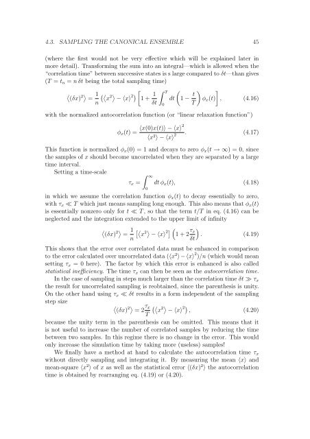
4.3. SAMPLING THE CANONICAL ENSEMBLE 45
(where the first would not be very effective which will be explained later in
more detail). Transforming the sum into an integral—which is allowed when the
“correlation time” between successive states is s large compared to δt—than gives
(T = tn = n δt being the total sampling time)
2
(δx) = 1 2
x
n
− 〈x〉
2
1 + 1
δt
T
0
dt 1 − t
φx(t) , (4.16)
T
with the normalized autocorrelation function (or “linear relaxation function”)
φx(t) =
〈x(0)x(t)〉 − 〈x〉2
〈x 2 〉 − 〈x〉 2 . (4.17)
This function is normalized φx(0) = 1 and decays to zero φx(t → ∞) = 0, since
the samples of x should become uncorrelated when they are separated by a large
time interval.
Setting a time-scale
∞
τx = dt φx(t), (4.18)
0
in which we assume the correlation function φx(t) to decay essentially to zero,
with τx ≪ T which just means sampling long enough. This also means that φx(t)
is essentially nonzero only for t ≪ T , so that the term t/T in eq. (4.16) can be
neglected and the integration extended to the upper limit of infinity
2
(δx) = 1 2
x
n
− 〈x〉
2
1 + 2 τx
. (4.19)
δt
This shows that the error over correlated data must be enhanced in comparison
to the error calculated over uncorrelated data (〈x2 〉−〈x〉 2 )/n (which would mean
setting τx = 0 here). The factor by which this error is enhanced is also called
statistical inefficiency. The time τx can then be seen as the autocorrelation time.
In the case of sampling in steps much larger than the correlation time δt ≫ τx
the result for uncorrelated sampling is reobtained, since the parenthesis is unity.
On the other hand using τx ≪ δt results in a form independent of the sampling
step size
2
(δx) = 2 τx 2
x − 〈x〉 2 , (4.20)
T
because the unity term in the parenthesis can be omitted. This means that it
is not useful to increase the number of correlated samples by reducing the time
between two samples. In this regime there is no change in the error. This would
only increase the simulation time by taking more (useless) samples!
We finally have a method at hand to calculate the autocorrelation time τx
without directly sampling and integrating it. By measuring the mean 〈x〉 and
mean-square 〈x 2 〉 of x as well as the statistical error 〈(δx) 2 〉 the autocorrelation
time is obtained by rearranging eq. (4.19) or (4.20).