Polymers in Confined Geometry.pdf

3.3. ANALYTICAL RESULTS 35
x 2 (s/L)
1.5e-05
1e-05
5e-06
0
0
0.2
Integral ansatz
Series ansatz
0.4
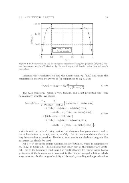
Figure 3.6: Comparison of the mean-square undulations along the polymer x 2 (s/L) versus
the contour length s/L obtained by Fourier integral and Fourier series (‘tracked ends’)
calculation.
Inserting this transformation into the Hamiltonian eq. (3.20) and using the
equipartition theorem we arrives at (in comparison to eq. (3.25))
s/L
L
〈xkxk ′〉 = 〈ykyk ′〉 = δkk ′
2
lp
0.6
0.8
1
.
k4 −4
(3.49)
+ 4ld The back-transform—which is very tedious, and is not presented here—can
be calculated exactly. We obtain
〈x(s)x(s ′ )〉 = L2
2
ɛ
c 3
1
sinh
c cos c − cosh c sin c
cos 2c − cosh 2c
· cosh(c − sc) sin(c − sc) sinh s ′ c cos s ′ c
+ sinh(c − sc) cos(c − sc) cosh s ′ c sin s ′ c
+ sinh c cos c + cosh c sin c
· cosh(c − sc) sin(c − sc) cosh s ′ c sin s ′ c
− sinh(c − sc) cos(c − sc) sinh s ′ c cos s ′ c
1
,
(3.50)
which is valid for s > s ′ , using besides the dimensionless parameters ɛ and c,
the abbreviations sc = s/ld and s ′ c = s ′ /ld. For further calculations this is a
very inconvenient expression. To obtain more results an algebraic program like
mathematica should be used.
For s = s ′ the mean-square undulations are obtained, which is compared to
eq. (3.27) in figure 3.6. The results for the inner part of the polymer are identical.
Due to the boundary conditions, the result obtained by Fourier series has to
go to zero at the boundaries, in contrast to the Fourier integral solution, which
stays constant. In the range of validity of the weakly-bending rod approximation