Polymers in Confined Geometry.pdf

More documents

Recommendations

Info

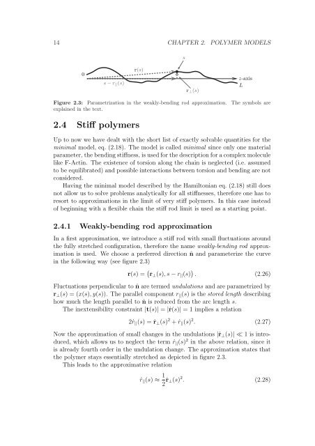
14 CHAPTER 2. POLYMER MODELS 0 s − r ||(s) r(s) s r⊥(s) z-axis L Figure 2.3: Parametrization in the weakly-bending rod approximation. The symbols are explained in the text. 2.4 Stiff polymers Up to now we have dealt with the short list of exactly solvable quantities for the minimal model, eq. (2.18). The model is called minimal since only one material parameter, the bending stiffness, is used for the description for a complex molecule like F-Actin. The existence of torsion along the chain is neglected (i.e. assumed to be equilibrated) and possible interactions between torsion and bending are not considered. Having the minimal model described by the Hamiltonian eq. (2.18) still does not allow us to solve problems analytically for all stiffnesses, therefore one has to resort to approximations in the limit of very stiff polymers. In this case instead of beginning with a flexible chain the stiff rod limit is used as a starting point. 2.4.1 Weakly-bending rod approximation In a first approximation, we introduce a stiff rod with small fluctuations around the fully stretched configuration, therefore the name weakly-bending rod approximation is used. We choose a preferred direction ˆn and parameterize the curve in the following way (see figure 2.3) r(s) = r⊥(s), s − r||(s) . (2.26) Fluctuations perpendicular to ˆn are termed undulations and are parametrized by r⊥(s) = (x(s), y(s)). The parallel component r||(s) is the stored length describing how much the length parallel to ˆn is reduced from the arc length s. The inextensibility constraint |t(s)| = |˙r(s)| = 1 implies a relation 2 ˙r||(s) = ˙r⊥(s) 2 + ˙r||(s) 2 . (2.27) Now the approximation of small changes in the undulations |˙r⊥(s)| ≪ 1 is introduced, which allows us to neglect the term ˙r||(s) 2 in the above relation, since it is already fourth order in the undulation change. The approximation states that the polymer stays essentially stretched as depicted in figure 2.3. This leads to the approximative relation ˙r||(s) ≈ 1 2 ˙r⊥(s) 2 . (2.28)
2.5. REAL CHAINS 15 no overhangs allowed |r⊥(s)| too large z-axis Figure 2.4: Overhangs are and large changes in |r⊥(s)| are not allowed Note that this implies that ˙r|| is non-negative or in other words that overhangs, as shown in figure 2.4, are not allowed. The derivative ¨r||(s) 2 1 d˙r⊥(s) ≈ 2 2 2 = ds ˙r⊥(s) · ¨r⊥(s) 2 (2.29) is already anharmonic and can therefore be neglected. Why this term does not contribute is easily seen in Fourier space. Due to the derivatives this term depends on the wave-vector as k 6 . Since in stiff polymers high frequency modes are suppressed by the bending energy, this term can be neglected. The term ¨r||(s) in the relation ¨r(s) 2 = ¨r⊥(s) 2 + ¨r||(s) 2 can be dropped ¨r(s) ≈ ¨r⊥(s). (2.30) This leads to the bending energy Hamiltonian in the weakly-bending rod approximation5 Hwb[r⊥(s)] = κ 2 L 0 ds ¨r⊥(s) 2 = κ 2 L 0 ds ¨x(s) 2 + ¨y(s) 2 . (2.31) Now the inextensibility constraint is implicitly, i.e. automatically, fulfilled. The path-integral for the partition sum, eq. (2.19), has been simplified, since the inextensibility constraint in weakly-bending rod approximation leaves only two independent components. This approximation is also called Monge-representation to indicate the chosen parametrization. The single valued contour is parametrized in reference to a reference line by the undulations 6 . 2.5 Real chains We have dealt so far with idealized chains represented by segments or a continuous space curve, allowed to interpenetrate each other. Therefore these models are 5In classical elasticity theory the energy of a weakly-bending rod has exactly the same form as this Hamiltonian (cf. [23]). 6In differential geometry the Monge-representation is used to parametrize single-valued planes by a ‘hight’ over a reference plane.
Page 1 and 2: Diploma Thesis Polymers in Confined
Page 3: TMTOWTDI—There’s More Than One
Page 7 and 8: Contents 1 Introduction 1 2 Polymer
Page 9 and 10: Chapter 1 Introduction Polymers are
Page 11 and 12: (a) λ-DNA (b) T2-DNA Figure 1.2: A
Page 13 and 14: Chapter 2 Polymer models This chapt
Page 15 and 16: 2.2. IDEAL PHANTOM CHAIN 7 configur
Page 17 and 18: 2.3. SEMI-FLEXIBLE POLYMERS 9 In th
Page 19 and 20: 2.3. SEMI-FLEXIBLE POLYMERS 11 to i
Page 21: 2.3. SEMI-FLEXIBLE POLYMERS 13 for
Page 25 and 26: 2.5. REAL CHAINS 17 Figure 2.5: Sna
Page 27 and 28: 2.5. REAL CHAINS 19 ln R cases intr
Page 29 and 30: Chapter 3 Polymers in confined geom
Page 31 and 32: 3.2. SCALING RELATIONS 23 using eq.
Page 33 and 34: 3.2. SCALING RELATIONS 25 b a d R |
Page 35 and 36: 3.3. ANALYTICAL RESULTS 27 The mean
Page 37 and 38: 3.3. ANALYTICAL RESULTS 29 From thi
Page 39 and 40: 3.3. ANALYTICAL RESULTS 31 a consta
Page 41 and 42: 3.3. ANALYTICAL RESULTS 33 the proj
Page 43 and 44: 3.3. ANALYTICAL RESULTS 35 x 2 (s/
Page 45 and 46: Chapter 4 Simulation methods This c
Page 47 and 48: 4.3. SAMPLING THE CANONICAL ENSEMBL
Page 55 and 56: 4.4. SIMULATION OF UNCONFINED WORM-
Page 57 and 58: 4.4. SIMULATION OF UNCONFINED WORM-
Page 59 and 60: 4.5. SIMULATION OF CONFINED WORM-LI
Page 61 and 62: 4.6. SAMPLED QUANTITIES AND THEIR R
Page 63 and 64: 4.6. SAMPLED QUANTITIES AND THEIR R
Page 65 and 66: Chapter 5 Simulation results In thi
Page 67 and 68: 5.2. THE HARMONIC POTENTIAL 59 ˆt
Page 69 and 70: 5.2. THE HARMONIC POTENTIAL 61 5.2.
Page 71 and 72: 5.2. THE HARMONIC POTENTIAL 63 beha
Page 73 and 74:
5.2. THE HARMONIC POTENTIAL 65 R 2
Page 75 and 76:
5.2. THE HARMONIC POTENTIAL 67 R 2
Page 77 and 78:
5.2. THE HARMONIC POTENTIAL 69 R
Page 79 and 80:
5.2. THE HARMONIC POTENTIAL 71 p(R)
Page 81 and 82:
5.3. THE HARD WALLS 73 〈Ra〉 1 0
Page 83 and 84:
Chapter 6 Conclusion Emerging from
Page 85 and 86:
Appendix A Discrete worm-like chain
Page 87 and 88:
which, after taking all the derivat
Page 89 and 90:
Appendix B Calculation for the conf
Page 91 and 92:
B.2. END-TO-END DISTANCE CORRELATIO
Page 93 and 94:
B.3. PARALLEL END-TO-END DISTANCE C
Page 95 and 96:
Glossary L filament length lp persi
Page 97 and 98:
Bibliography [1] M. Abramowitz and
Page 99 and 100:
BIBLIOGRAPHY 91 [29] P. L’Ecuyer.
Page 101:
:wq
show all

Polymers in Confined Geometry.pdf

Create successful ePaper yourself

Delete template?

Save as template?