Polymers in Confined Geometry.pdf

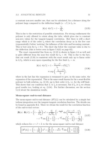
3.3. ANALYTICAL RESULTS 31
a constant non-zero smaller one, that can be calculated, for a distance along the
polymer large compared to the deflection length |s − s ′ | ≫ ld, to
〈t(s) · t(s ′ )〉 = 1 − ld
. (3.35)
2lp
This is due to the restriction of possible orientations. For strong confinement the
polymer is only allowed to orient along the tube, which gives rise to constant
non-zero values for the tangent-tangent correlation. But there is still a short
range which is of the order ld where the correlation decay as in the free case
(exponentially) before ‘noticing’ the influence of the tube and becoming constant.
This is best seen for ld = 0.1. The short dip below the constant value is due to
the deflection (this is better seen in figure 5.4(d) on page 62).
The exact exponential line from eq. (2.12) is shown in figure 3.4 as well and
is quite different from the near free result for ld = 10. This is due to the fact,
that our result (3.34) is consistent with the exact result only up to linear order
in L/lp, which is seen upon expanding for the free limit ld → ∞
〈t(s) · t(s ′ )〉 = 1 − |s − s′ |
lp
≈ exp − |s − s′ |
lp
+ O(l −1
d )
,
(3.36)
where in the last line the expansion is resummed to give, in the same order, the
expansion of the exponential. This is the same result known for the a semi-flexible
polymer in bulk solution, eq. (2.12), up to first order L/lp, i.e. for the stiff limit.
This shows that our condition that L ≪ lp is necessary, but if lp ≫ ld we obtain
good results too, looking at eq. (3.34). For further discussion, see the section
5.2.2 about the simulation results.
Mean-square end-to-end distance
The mean-square end-to-end distance 〈R 2 (L)〉 can be calculated by a simple but
tedious integration over the tangent-tangent correlation function. The details can
be found in appendix B.2. There we obtain the result for the correlation function
of the end-to-end vectors
〈R(s) · R(s ′ )〉 =
1 − ld
ss
2 lp
′ + l3 d
2 √ 2 lp
s
− l − e d sin
s
ld
+ π
4
e − |s−s′
|
′ |s − s |
ld sin
ld
s′ ′
− s l − e d sin +
ld
π
4
+ π
4
+ 1
√ 2
,
(3.37)
which reduces for s = s ′ = L to the the mean-square end-to-end distance
2
R (L) = 1 − ld
L
2 lp
2 + l3
d
1 −
2 lp
√
L
− L
l 2 e d sin +
ld
π
. (3.38)
4