Polymers in Confined Geometry.pdf

More documents

Recommendations

Info

16 CHAPTER 2. POLYMER MODELS frequently called phantom chains. But in reality polymers are charged objects in a solution surrounded by charges. Therefore the interaction between the polymer segments is very complex and depends on the solution. But often one is entitled to replace these interaction by a simplified hard core interaction. The next step in the direction of a more realistic model is then to incorporate self-avoidance effects as a steep short-ranged repulsive potential between the segments (of the order of the microscopic polymer thickness). The polymer is not allowed to intersect with itself 7 . For detailed description of models with ‘realistic’ features confer e.g. [39]. The influence of the self-avoidance/excluded volume is visible in particular for flexible/long (i.e. a large ratio of L/lp) chains since they fold back and forth freely, therefore crossing themselves very often. As a result the polymer will tend to be more extended than a phantom chain due to the reduced number of allowed configurations (entropic penalty) in the strongly collapsed state. In contrast for stiff polymers the effect is mostly negligible since it is unlikely for them to fold back onto themselves. At variance with the description of the ideal phantom chain as a random walk, the self-avoiding random walk can be used to investigate the properties of these chains. But we want to focus on the derivation of the basic scaling relation for the end-to-end distance. The considerations of the “entropic penalty” can be used to derive a scaling relation similar to eq. (2.6) for the ideal chain. This argument dates back to P. Flory and is described in detail in [8] and [39]. It considers a correction to the free energy of the ideal chain, eq. (2.8), that is due to the excluded volume which, in turn, depends on the number of monomer-monomer contacts. Let v be the mean volume occupied by a monomer depending on the segment length b and the thickness of the chain d. The monomer density φ of a chain of linear size R which occupies a sphere of about the volume R 3 is φ ∼ Nv . (2.32) R3 The entropy loss for an exclusion is of order kBT for each degree of freedom (equipartition theorem). Since there are N monomers the free energy correction is F ∼ kBT v N 2 . (2.33) R3 Additionally using the free energy of the ideal chain, eq. (2.8), one can minimize the sum of these contributions with respect to the end-to-end distance R. We obtain the scaling result R ∼ (b 2 v) 1/5 N 3/5 . (2.34) 7 There exists a so called θ-temperature (depending on the solution) where the segmentsegment interaction is exactly balanced by effects from the surrounding solution. Then the description of an ideal chain is valid.
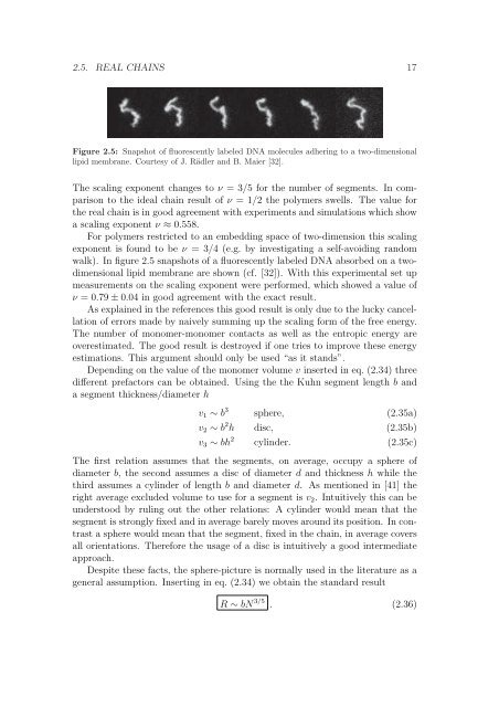
2.5. REAL CHAINS 17 Figure 2.5: Snapshot of fluorescently labeled DNA molecules adhering to a two-dimensional lipid membrane. Courtesy of J. Rädler and B. Maier [32]. The scaling exponent changes to ν = 3/5 for the number of segments. In comparison to the ideal chain result of ν = 1/2 the polymers swells. The value for the real chain is in good agreement with experiments and simulations which show a scaling exponent ν ≈ 0.558. For polymers restricted to an embedding space of two-dimension this scaling exponent is found to be ν = 3/4 (e.g. by investigating a self-avoiding random walk). In figure 2.5 snapshots of a fluorescently labeled DNA absorbed on a twodimensional lipid membrane are shown (cf. [32]). With this experimental set up measurements on the scaling exponent were performed, which showed a value of ν = 0.79 ± 0.04 in good agreement with the exact result. As explained in the references this good result is only due to the lucky cancellation of errors made by naively summing up the scaling form of the free energy. The number of monomer-monomer contacts as well as the entropic energy are overestimated. The good result is destroyed if one tries to improve these energy estimations. This argument should only be used “as it stands”. Depending on the value of the monomer volume v inserted in eq. (2.34) three different prefactors can be obtained. Using the the Kuhn segment length b and a segment thickness/diameter h v1 ∼ b 3 sphere, (2.35a) v2 ∼ b 2 h disc, (2.35b) v3 ∼ bh 2 cylinder. (2.35c) The first relation assumes that the segments, on average, occupy a sphere of diameter b, the second assumes a disc of diameter d and thickness h while the third assumes a cylinder of length b and diameter d. As mentioned in [41] the right average excluded volume to use for a segment is v2. Intuitively this can be understood by ruling out the other relations: A cylinder would mean that the segment is strongly fixed and in average barely moves around its position. In contrast a sphere would mean that the segment, fixed in the chain, in average covers all orientations. Therefore the usage of a disc is intuitively a good intermediate approach. Despite these facts, the sphere-picture is normally used in the literature as a general assumption. Inserting in eq. (2.34) we obtain the standard result R ∼ bN 3/5 . (2.36)
Page 1 and 2: Diploma Thesis Polymers in Confined
Page 3: TMTOWTDI—There’s More Than One
Page 7 and 8: Contents 1 Introduction 1 2 Polymer
Page 9 and 10: Chapter 1 Introduction Polymers are
Page 11 and 12: (a) λ-DNA (b) T2-DNA Figure 1.2: A
Page 13 and 14: Chapter 2 Polymer models This chapt
Page 15 and 16: 2.2. IDEAL PHANTOM CHAIN 7 configur
Page 17 and 18: 2.3. SEMI-FLEXIBLE POLYMERS 9 In th
Page 19 and 20: 2.3. SEMI-FLEXIBLE POLYMERS 11 to i
Page 21 and 22: 2.3. SEMI-FLEXIBLE POLYMERS 13 for
Page 23: 2.5. REAL CHAINS 15 no overhangs al
Page 27 and 28: 2.5. REAL CHAINS 19 ln R cases intr
Page 29 and 30: Chapter 3 Polymers in confined geom
Page 31 and 32: 3.2. SCALING RELATIONS 23 using eq.
Page 33 and 34: 3.2. SCALING RELATIONS 25 b a d R |
Page 35 and 36: 3.3. ANALYTICAL RESULTS 27 The mean
Page 37 and 38: 3.3. ANALYTICAL RESULTS 29 From thi
Page 39 and 40: 3.3. ANALYTICAL RESULTS 31 a consta
Page 41 and 42: 3.3. ANALYTICAL RESULTS 33 the proj
Page 43 and 44: 3.3. ANALYTICAL RESULTS 35 x 2 (s/
Page 45 and 46: Chapter 4 Simulation methods This c
Page 47 and 48: 4.3. SAMPLING THE CANONICAL ENSEMBL
Page 55 and 56: 4.4. SIMULATION OF UNCONFINED WORM-
Page 57 and 58: 4.4. SIMULATION OF UNCONFINED WORM-
Page 59 and 60: 4.5. SIMULATION OF CONFINED WORM-LI
Page 61 and 62: 4.6. SAMPLED QUANTITIES AND THEIR R
Page 63 and 64: 4.6. SAMPLED QUANTITIES AND THEIR R
Page 65 and 66: Chapter 5 Simulation results In thi
Page 67 and 68: 5.2. THE HARMONIC POTENTIAL 59 ˆt
Page 69 and 70: 5.2. THE HARMONIC POTENTIAL 61 5.2.
Page 71 and 72: 5.2. THE HARMONIC POTENTIAL 63 beha
Page 73 and 74: 5.2. THE HARMONIC POTENTIAL 65 R 2
Page 75 and 76:
5.2. THE HARMONIC POTENTIAL 67 R 2
Page 77 and 78:
5.2. THE HARMONIC POTENTIAL 69 R
Page 79 and 80:
5.2. THE HARMONIC POTENTIAL 71 p(R)
Page 81 and 82:
5.3. THE HARD WALLS 73 〈Ra〉 1 0
Page 83 and 84:
Chapter 6 Conclusion Emerging from
Page 85 and 86:
Appendix A Discrete worm-like chain
Page 87 and 88:
which, after taking all the derivat
Page 89 and 90:
Appendix B Calculation for the conf
Page 91 and 92:
B.2. END-TO-END DISTANCE CORRELATIO
Page 93 and 94:
B.3. PARALLEL END-TO-END DISTANCE C
Page 95 and 96:
Glossary L filament length lp persi
Page 97 and 98:
Bibliography [1] M. Abramowitz and
Page 99 and 100:
BIBLIOGRAPHY 91 [29] P. L’Ecuyer.
Page 101:
:wq
show all

Polymers in Confined Geometry.pdf

Create successful ePaper yourself

Delete template?

Save as template?