Polymers in Confined Geometry.pdf

More documents

Recommendations

Info

52 CHAPTER 4. SIMULATION METHODS detail will be the cylindrical symmetric harmonic potential as already introduced in eq. (3.20). The accuracy of this approximation and how to relate it to the other potentials will be discussed in section 5. 4.5.1 Harmonic potential The configuration energy function ∆e corresponding to eq. (4.25) is given by the discretized version of eq. (3.20) N−1 ∆e = βH ({ti}) = −k ˆti · ˆti+1 + g 2 i=1 N 2 xi + y 2 i , (4.29) such that we now need the tangents and the positions of the beads in the simulation. The latter can be directly calculated from the tangents, but storing them is faster. We have to relate the prefactor g to the Odijk deflection length ld by discretizing the harmonic potential part of eq. (3.20). Additionally one has to use dimensionless units in the simulation. Hence all positions are measured in units of the segment length l γ 2 L 0 ds x(s) 2 + y(s) 2 = γl3 2 → γl3 2 g/2β Nl 0 ds l i=0 x(s) l 2 2 y(s) + l N 2 xi + y 2 i , (4.30) where xi, yi are normalized by the segment length l = L/N. Upon using the one finds definition ld := (4κ/γ) 1 4 ⇒ γ = 4κ/l 4 d g = βγl 3 = 4βκl3 l 4 d i=0 (2.20) = 4lpl 3 l 4 d = 4c4 N 3 . (4.31) ɛ The actual parameter used for the simulations is the collision parameter c as defined in eq. (3.3). With these prerequisites the simulation can be implemented straightforwardly. Only one additional MC move must be added since the space is not isotropic anymore. Now global movements of the polymer perpendicular to the tube axis must be attempted. This can be implemented by using a virtual segment ‘zero’. If this is randomly selected, all positions are shifted by a random amount out of ±∆r⊥. The detailed balance condition is therefore obeyed. This maximum shift is, along with the maximal rotation angle δα, adjusted in the initial simulation phase. The z-position of the first bead can be kept fixed, since there is still the rotational symmetry around the tube/z-axis.
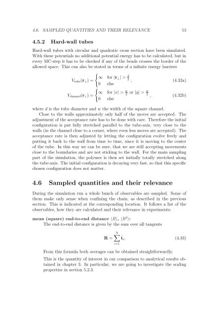
4.6. SAMPLED QUANTITIES AND THEIR RELEVANCE 53 4.5.2 Hard-wall tubes Hard-wall tubes with circular and quadratic cross section have been simulated. With these potentials no additional potential energy has to be calculated, but in every MC-step it has to be checked if any of the beads crosses the border of the allowed space. This can also be stated in terms of a infinite energy barriers ∞ for |r⊥| > Vtube(r⊥) = d 2 , (4.32a) Vchannel(r⊥) = 0 else ∞ for |x| > w 2 0 else or |y| > w 2 , (4.32b) where d is the tube diameter and w the width of the square channel. Close to the walls approximately only half of the moves are accepted. The adjustment of the acceptance rate has to be done with care. Therefore the initial configuration is put fully stretched parallel to the tube-axis, very close to the walls (in the channel close to a corner, where even less moves are accepted). The acceptance rate is then adjusted by letting the configuration evolve freely and putting it back to the wall from time to time, since it is moving to the center of the tube. In this way we can be sure, that we are still accepting movements close to the boundaries and are not sticking to the wall. For the main sampling part of the simulation, the polymer is then set initially totally stretched along the tube-axis. The initial configuration is decaying very fast, so that this specific chosen configuration does not matter. 4.6 Sampled quantities and their relevance During the simulation run a whole bunch of observables are sampled. Some of them make only sense when confining the chain, as described in the previous section. This is indicated at the corresponding location. It follows a list of the observables, how they are calculated and their relevance in experiments: mean (square) end-to-end distance 〈R〉, 〈R 2 〉: The end-to-end distance is given by the sum over all tangents R = N ˆti. (4.33) From this formula both averages can be obtained straightforwardly. i=1 This is the quantity of interest in our comparison to analytical results obtained in chapter 3. In particular, we are going to investigate the scaling properties in section 5.2.3.
Page 1 and 2:
Diploma Thesis Polymers in Confined
Page 3:
TMTOWTDI—There’s More Than One
Page 7 and 8:
Contents 1 Introduction 1 2 Polymer
Page 9 and 10: Chapter 1 Introduction Polymers are
Page 11 and 12: (a) λ-DNA (b) T2-DNA Figure 1.2: A
Page 13 and 14: Chapter 2 Polymer models This chapt
Page 15 and 16: 2.2. IDEAL PHANTOM CHAIN 7 configur
Page 17 and 18: 2.3. SEMI-FLEXIBLE POLYMERS 9 In th
Page 19 and 20: 2.3. SEMI-FLEXIBLE POLYMERS 11 to i
Page 21 and 22: 2.3. SEMI-FLEXIBLE POLYMERS 13 for
Page 23 and 24: 2.5. REAL CHAINS 15 no overhangs al
Page 25 and 26: 2.5. REAL CHAINS 17 Figure 2.5: Sna
Page 27 and 28: 2.5. REAL CHAINS 19 ln R cases intr
Page 29 and 30: Chapter 3 Polymers in confined geom
Page 31 and 32: 3.2. SCALING RELATIONS 23 using eq.
Page 33 and 34: 3.2. SCALING RELATIONS 25 b a d R |
Page 35 and 36: 3.3. ANALYTICAL RESULTS 27 The mean
Page 37 and 38: 3.3. ANALYTICAL RESULTS 29 From thi
Page 39 and 40: 3.3. ANALYTICAL RESULTS 31 a consta
Page 41 and 42: 3.3. ANALYTICAL RESULTS 33 the proj
Page 43 and 44: 3.3. ANALYTICAL RESULTS 35 x 2 (s/
Page 45 and 46: Chapter 4 Simulation methods This c
Page 47 and 48: 4.3. SAMPLING THE CANONICAL ENSEMBL
Page 55 and 56: 4.4. SIMULATION OF UNCONFINED WORM-
Page 57 and 58: 4.4. SIMULATION OF UNCONFINED WORM-
Page 59: 4.5. SIMULATION OF CONFINED WORM-LI
Page 63 and 64: 4.6. SAMPLED QUANTITIES AND THEIR R
Page 65 and 66: Chapter 5 Simulation results In thi
Page 67 and 68: 5.2. THE HARMONIC POTENTIAL 59 ˆt
Page 69 and 70: 5.2. THE HARMONIC POTENTIAL 61 5.2.
Page 71 and 72: 5.2. THE HARMONIC POTENTIAL 63 beha
Page 73 and 74: 5.2. THE HARMONIC POTENTIAL 65 R 2
Page 75 and 76: 5.2. THE HARMONIC POTENTIAL 67 R 2
Page 77 and 78: 5.2. THE HARMONIC POTENTIAL 69 R
Page 79 and 80: 5.2. THE HARMONIC POTENTIAL 71 p(R)
Page 81 and 82: 5.3. THE HARD WALLS 73 〈Ra〉 1 0
Page 83 and 84: Chapter 6 Conclusion Emerging from
Page 85 and 86: Appendix A Discrete worm-like chain
Page 87 and 88: which, after taking all the derivat
Page 89 and 90: Appendix B Calculation for the conf
Page 91 and 92: B.2. END-TO-END DISTANCE CORRELATIO
Page 93 and 94: B.3. PARALLEL END-TO-END DISTANCE C
Page 95 and 96: Glossary L filament length lp persi
Page 97 and 98: Bibliography [1] M. Abramowitz and
Page 99 and 100: BIBLIOGRAPHY 91 [29] P. L’Ecuyer.
Page 101: :wq
show all

Polymers in Confined Geometry.pdf

You also want an ePaper? Increase the reach of your titles

Delete template?

Save as template?