Polymers in Confined Geometry.pdf

More documents

Recommendations

Info

48 CHAPTER 4. SIMULATION METHODS where the prefactor k is related to the persistence length lp by eqs. (A.8) and (A.10). As input parameter for the simulation the flexibility ɛ is taken so that everything is measured in units of total length L (cf. eq. (3.2)). All output is normalized by L as well. This Hamiltonian is used to perform an off-lattice simulation where the polymer can orient without any restriction (cf. [25]). In a straightforward algorithm the polymer is represented by just its N segments, where the positions of the joints can be ignored as long as the polymer is unconfined. The basic steps are: 1. perform a random movement on a randomly chosen segment 2. calculate the change in configuration energy ∆e 3. accept/reject the move corresponding to the Metropolis algorithm (4. take samples after a specific number of steps) This three (four) basic steps are the essential part of the MC scheme. They will be discussed now in more detail. Step 1: The trial movement in the n-th MC-step is chosen by drawing a random number m to specify a segment to change ˆt (n) m → ˜t (n) m . The orientation is changed by a multiplication with a rotational matrix R l k , which is chosen out of a set that has been calculated in the initial phase of the simulation. The superscript l numbers one of the d spacial dimensions and k the specific matrix chosen from the set. It turned out to be optimal having 20 d equidistant discrete matrices (20 for each dimension) out of a maximal rotation angle ±δα/2. This angels must be tuned to give an overall acceptance rate of 25–50%. Detailed balance is obviously guaranteed: choosing a rotation matrix by first choosing one direction at random and than again randomly a specific rotation 6 . Thus this step is subsumed by—with random numbers m = 1, . . . , N, l = 1, . . . , d and k = 1, . . . , 20— ˜t (n) i = Rl k · ˆt (n) m for i = m ˆt (n) . (4.26) i for i = m One segment m is changed, where the orientation of all others is kept fixed as shown in figure 4.1. An alternative approach to the simulation in two dimension is by noting that the polymer configuration is fully specified by knowing the angles θi between each segment and a fixed global direction (see figure 4.1). The simulation can than be build on trial moves changing these angles, i.e. taking a random change on 6 E.g. it would be wrong to use in each step a rotation in all d-direction, when applying the rotation always in the same order. This is due to the non-commutativity of rotations, which breaks detailed balance in this case. But choosing the order of application randomly, again obeys detailed balance, but has an unnecessary calculation overhead.
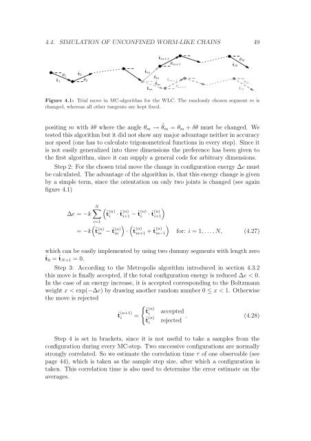
4.4. SIMULATION OF UNCONFINED WORM-LIKE CHAINS 49 ˆt1 θ1 ˆt2 θ2 ˆtm ˜tm Figure 4.1: Trial move in MC-algorithm for the WLC. The randomly chosen segment m is changed, whereas all other tangents are kept fixed. positing m with δθ where the angle θm → ˜ θm = θm + δθ must be changed. We tested this algorithm but it did not show any major advantage neither in accuracy nor speed (one has to calculate trigonometrical functions in every step). Since it is not easily generalized into three dimensions the preference has been given to the first algorithm, since it can supply a general code for arbitrary dimensions. Step 2: For the chosen trial move the change in configuration energy ∆e must be calculated. The advantage of the algorithm is, that this energy change is given by a simple term, since the orientation on only two joints is changed (see again figure 4.1) ∆e = −k N i=1 ˜t (n) i = −k ˜t (n) m − ˆt (n) m · · ˜t (n) i+1 − ˆt (n) i θm ˜θm ˆtm+1 · ˆt (n) i+1 ˆt (n) m+1 + ˆt (n) m−1 θm+1 ˆtm+1 θm+1 ˆtN θN ˆtN θN for: i = 1, . . . , N, (4.27) which can be easily implemented by using two dummy segments with length zero ˆt0 = ˆtN+1 = 0. Step 3: According to the Metropolis algorithm introduced in section 4.3.2 this move is finally accepted, if the total configuration energy is reduced ∆e < 0. In the case of an energy increase, it is accepted corresponding to the Boltzmann weight x < exp(−∆e) by drawing another random number 0 ≤ x < 1. Otherwise the move is rejected ˆt (n+1) i = ˜t (n) i accepted . (4.28) ˆt (n) i rejected Step 4 is set in brackets, since it is not useful to take a samples from the configuration during every MC-step. Two successive configurations are normally strongly correlated. So we estimate the correlation time τ of one observable (see page 44), which is taken as the sample step size, after which a configuration is taken. This correlation time is also used to determine the error estimate on the averages.
Page 1 and 2:
Diploma Thesis Polymers in Confined
Page 3:
TMTOWTDI—There’s More Than One
Page 7 and 8: Contents 1 Introduction 1 2 Polymer
Page 9 and 10: Chapter 1 Introduction Polymers are
Page 11 and 12: (a) λ-DNA (b) T2-DNA Figure 1.2: A
Page 13 and 14: Chapter 2 Polymer models This chapt
Page 15 and 16: 2.2. IDEAL PHANTOM CHAIN 7 configur
Page 17 and 18: 2.3. SEMI-FLEXIBLE POLYMERS 9 In th
Page 19 and 20: 2.3. SEMI-FLEXIBLE POLYMERS 11 to i
Page 21 and 22: 2.3. SEMI-FLEXIBLE POLYMERS 13 for
Page 23 and 24: 2.5. REAL CHAINS 15 no overhangs al
Page 25 and 26: 2.5. REAL CHAINS 17 Figure 2.5: Sna
Page 27 and 28: 2.5. REAL CHAINS 19 ln R cases intr
Page 29 and 30: Chapter 3 Polymers in confined geom
Page 31 and 32: 3.2. SCALING RELATIONS 23 using eq.
Page 33 and 34: 3.2. SCALING RELATIONS 25 b a d R |
Page 35 and 36: 3.3. ANALYTICAL RESULTS 27 The mean
Page 37 and 38: 3.3. ANALYTICAL RESULTS 29 From thi
Page 39 and 40: 3.3. ANALYTICAL RESULTS 31 a consta
Page 41 and 42: 3.3. ANALYTICAL RESULTS 33 the proj
Page 43 and 44: 3.3. ANALYTICAL RESULTS 35 x 2 (s/
Page 45 and 46: Chapter 4 Simulation methods This c
Page 47 and 48: 4.3. SAMPLING THE CANONICAL ENSEMBL
Page 55: 4.4. SIMULATION OF UNCONFINED WORM-
Page 59 and 60: 4.5. SIMULATION OF CONFINED WORM-LI
Page 61 and 62: 4.6. SAMPLED QUANTITIES AND THEIR R
Page 63 and 64: 4.6. SAMPLED QUANTITIES AND THEIR R
Page 65 and 66: Chapter 5 Simulation results In thi
Page 67 and 68: 5.2. THE HARMONIC POTENTIAL 59 ˆt
Page 69 and 70: 5.2. THE HARMONIC POTENTIAL 61 5.2.
Page 71 and 72: 5.2. THE HARMONIC POTENTIAL 63 beha
Page 73 and 74: 5.2. THE HARMONIC POTENTIAL 65 R 2
Page 75 and 76: 5.2. THE HARMONIC POTENTIAL 67 R 2
Page 77 and 78: 5.2. THE HARMONIC POTENTIAL 69 R
Page 79 and 80: 5.2. THE HARMONIC POTENTIAL 71 p(R)
Page 81 and 82: 5.3. THE HARD WALLS 73 〈Ra〉 1 0
Page 83 and 84: Chapter 6 Conclusion Emerging from
Page 85 and 86: Appendix A Discrete worm-like chain
Page 87 and 88: which, after taking all the derivat
Page 89 and 90: Appendix B Calculation for the conf
Page 91 and 92: B.2. END-TO-END DISTANCE CORRELATIO
Page 93 and 94: B.3. PARALLEL END-TO-END DISTANCE C
Page 95 and 96: Glossary L filament length lp persi
Page 97 and 98: Bibliography [1] M. Abramowitz and
Page 99 and 100: BIBLIOGRAPHY 91 [29] P. L’Ecuyer.
Page 101: :wq
show all

Polymers in Confined Geometry.pdf

You also want an ePaper? Increase the reach of your titles

Delete template?

Save as template?