SEBAL - Dca.ufcg.edu.br

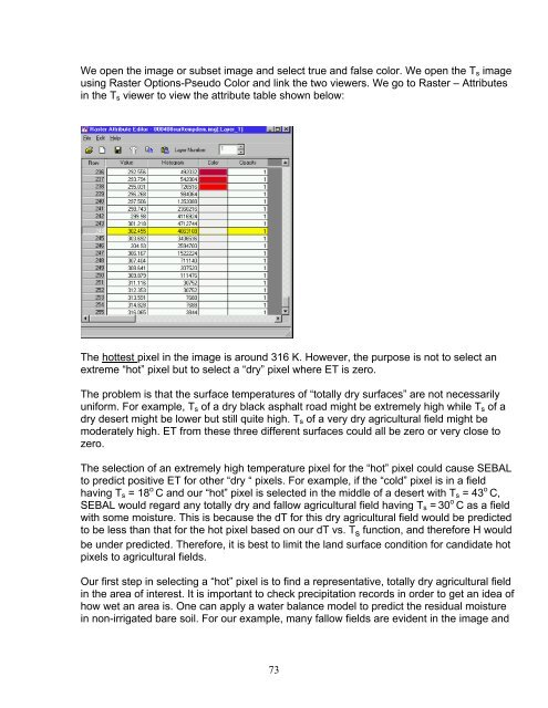
We open the image or subset image and select true and false color. We open the T s imageusing Raster Options-Pseudo Color and link the two viewers. We go to Raster – Attributesin the T s viewer to view the attribute table shown below:The hottest pixel in the image is around 316 K. However, the purpose is not to select anextreme “hot” pixel but to select a “dry” pixel where ET is zero.The problem is that the surface temperatures of “totally dry surfaces” are not necessarilyuniform. For example, T s of a dry black asphalt road might be extremely high while T s of adry desert might be lower but still quite high. T s of a very dry agricultural field might bemoderately high. ET from these three different surfaces could all be zero or very close tozero.The selection of an extremely high temperature pixel for the “hot” pixel could cause SEBALto predict positive ET for other “dry “ pixels. For example, if the “cold” pixel is in a fieldhaving T s = 18 o C and our “hot” pixel is selected in the middle of a desert with T s = 43 o C,SEBAL would regard any totally dry and fallow agricultural field having T s = 30 o C as a fieldwith some moisture. This is because the dT for this dry agricultural field would be predictedto be less than that for the hot pixel based on our dT vs. T s function, and therefore H wouldbe under predicted. Therefore, it is best to limit the land surface condition for candidate hotpixels to agricultural fields.Our first step in selecting a “hot” pixel is to find a representative, totally dry agricultural fieldin the area of interest. It is important to check precipitation records in order to get an idea ofhow wet an area is. One can apply a water balance model to predict the residual moisturein non-irrigated bare soil. For our example, many fallow fields are evident in the image and73