SEBAL - Dca.ufcg.edu.br

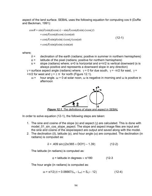
aspect of the land surface. SEBAL uses the following equation for computing cos θ (Duffieand Beckman, 1991):cosθ= sin( δ )sin( φ)cos(s)− sin( δ )cos( φ)sin(s)cos(γ )+ cos( δ )cos( φ)cos(s)cos(ω)+ cos( δ )sin( φ)sin(s)cos(γ )cos( ω)+ cos( δ )sin( φ)sin(s)sin(ω)(12-1)where;δ = declination of the earth (radians; positive in summer in northern hemisphere)φ = latitude of the pixel (radians; positive for northern hemisphere)s = slope (radians) where; s=0 is horizontal and s=π/2 is vertical downward (s isalways positive and represents a downward slope in any direction)γ = surface aspect angle (radians) where; γ = 0 for due south, γ = -π/2 for east, γ =+π/2 for west and γ = ± π for north (Figure 12.1).ω = hour angle. ω = 0 at solar noon, ω is negative in morning and ω is positive inafternoonFigure 12.1. The definitions of slope and aspect in SEBALIn order to solve equation (12-1), the following steps are taken:1. The sine and cosine of the slope (s) and aspect (γ) are calculated. This is done withmodel_01_sin_cos_slope_aspect. The slope and aspect image files are input andthe sine and cosine of the slope/aspect are output and saved along with the model.2. The declination (δ), latitude (φ), and hour angle (ω) are computed. The declination (inradians) is computed as:δ = .409 sin{(2π/365 × DOY) – 1.39} (12-2)The latitude (in radians) is computed as:φ = latitude in degrees × π/180 (12-3The hour angle (in radians) is computed as:ω = π/12{(t + 0.06667(L z - L m ) + S c ) - 12} (12-4)94