SEBAL - Dca.ufcg.edu.br

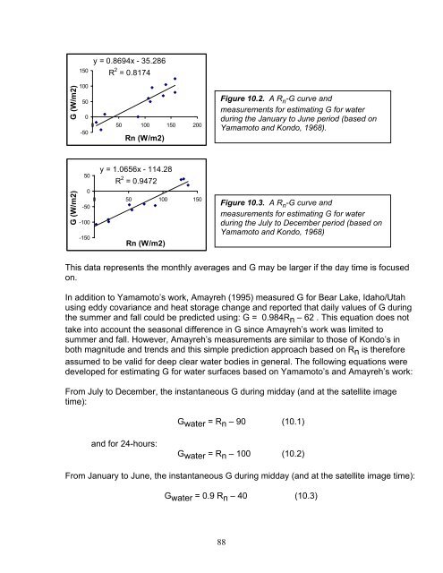
150y = 0.8694x - 35.286R 2 = 0.8174G (W/m2)1005000 50 100 150 200-50Rn (W/m2)Figure 10.2. A R n -G curve andmeasurements for estimating G for waterduring the January to June period (based onYamamoto and Kondo, 1968).G (W/m2)y = 1.0656x - 114.28R 2 = 0.94725000 50 100 150-50-100-150Rn (W/m2)Figure 10.3. A R n -G curve andmeasurements for estimating G for waterduring the July to December period (based onYamamoto and Kondo, 1968)This data represents the monthly averages and G may be larger if the day time is focusedon.In addition to Yamamoto’s work, Amayreh (1995) measured G for Bear Lake, Idaho/Utahusing eddy covariance and heat storage change and reported that daily values of G duringthe summer and fall could be predicted using: G = 0.984Rn – 62 . This equation does nottake into account the seasonal difference in G since Amayreh’s work was limited tosummer and fall. However, Amayreh’s measurements are similar to those of Kondo’s inboth magnitude and trends and this simple prediction approach based on Rn is thereforeassumed to be valid for deep clear water bodies in general. The following equations weredeveloped for estimating G for water surfaces based on Yamamoto’s and Amayreh’s work:From July to December, the instantaneous G during midday (and at the satellite imagetime):Gwater = Rn – 90 (10.1)and for 24-hours:Gwater = Rn – 100 (10.2)From January to June, the instantaneous G during midday (and at the satellite image time):Gwater = 0.9 Rn – 40 (10.3)88