SEBAL - Dca.ufcg.edu.br

More documents

Recommendations

Info

Remote sensing has great potential for improving irrigation management, along withother types of water management by providing ET estimations for large land surfaceareas using a minimal amount of ground data.3. OBJECTIVESThis manual explains a remote image-processing model for predicting ET termed SEBAL(Surface Energy Balance Algorithm for Land). SEBAL calculates ET through a series ofcomputations that generate: net surface radiation, soil heat flux, and sensible heat flux tothe air. By subtracting the soil heat flux and sensible heat flux from the net radiation at thesurface we are left with a “residual” energy flux that is used for evapotranspiration (i.e.energy that is used to convert the liquid water into water vapor). This manual describes thetheoretical basis of SEBAL using images from Landsat 5 and 7 satellites. However, thetheory is independent of the satellite type and this manual could be applied to other satelliteimages if used with appropriate coefficients.4. WHO CAN USE THIS MANUAL?The user of this manual should have background knowledge in hydrologic science orengineering and environmental physics (theories of mass and momentum transfer), as wellas solar radiation physics. SEBAL was developed for use with ERDAS IMAGINE’s ModelMaker tool and experience with this software is a prerequisite. As with any computer model,only knowledgeable users who understand the theory and who can consistently recognizethe reliability of the computations should use SEBAL. As will be shown, it is also importantthat the user be familiar with the area being studied and has some “on the ground”knowledge of land use and topography for the area of interest. Following is a list of usefulreferences, which provide a good background of the scientific methods used in SEBAL:1. Monteith, J. L. and Unsworth, M. H. (1990). Principles of Environmental Physics,Second Edition, Butterworth Heinemann. ISBN 0-7131-2931- X2. Campbell, G. S. and Norman, J. M. (1998). An Introduction To EnvironmentalBiophysics, Second Edition, Springer. ISBN 0-387-94937-23. Allen, R. G., Pereira, L., Raes, D., and Smith, M. (1998). CropEvapotranspiration, Food and Agriculture Organization of the United Nations,Rome, Italy. ISBN 92-5-104219-5. 290 p.4. Allen, R.G. (2000). REF-ET: Reference Evapotranspiration Calculation Softwarefor FAO and ASCE Standardized Equations, University of Idaho.www.kimberly.uidaho.edu/ref-et/8
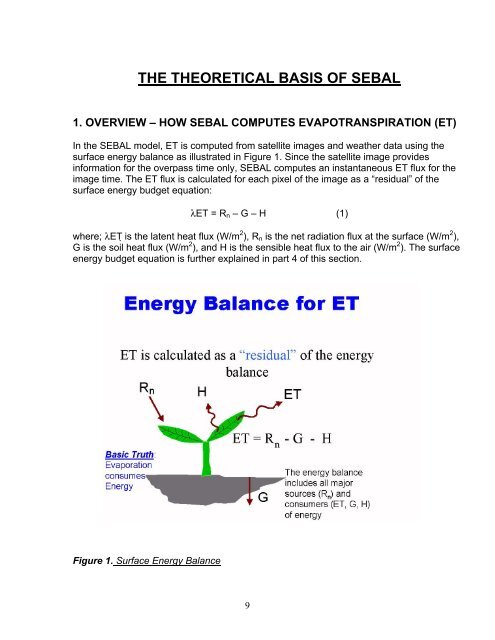
THE THEORETICAL BASIS OF SEBAL1. OVERVIEW – HOW SEBAL COMPUTES EVAPOTRANSPIRATION (ET)In the SEBAL model, ET is computed from satellite images and weather data using thesurface energy balance as illustrated in Figure 1. Since the satellite image providesinformation for the overpass time only, SEBAL computes an instantaneous ET flux for theimage time. The ET flux is calculated for each pixel of the image as a “residual” of thesurface energy budget equation:λET = R n – G – H (1)where; λET is the latent heat flux (W/m 2 ), R n is the net radiation flux at the surface (W/m 2 ),G is the soil heat flux (W/m 2 ), and H is the sensible heat flux to the air (W/m 2 ). The surfaceenergy budget equation is further explained in part 4 of this section.Figure 1. Surface Energy Balance9
Page 1 and 2: SEBALSurface Energy Balance Algorit
Page 3 and 4: 6. Tables for surface albedo comput
Page 5 and 6: δ declination of the earth radians
Page 7: INTRODUCTION1. BACKGROUNDLand manag
Page 11 and 12: The surface emissivity is the ratio
Page 13 and 14: • Reference evapotranspiration, E
Page 15 and 16: Figure 3. Flow Chart of the Net Sur
Page 17 and 18: 2. The reflectivity for each band (
Page 19 and 20: and ET are specified for the two ex
Page 21 and 22: To complete step 2, model F06_surfa
Page 23 and 24: D. Choosing the “Hot” and “Co
Page 25 and 26: irrigated crops near Kimberly, Idah
Page 27 and 28: where; u * is the friction velocity
Page 29 and 30: Weather stationu, z x, z om, u *H f
Page 31 and 32: Note: An alternative method used by
Page 33 and 34: where;⎛ 2 ⎞⎜1+ x(0.1m)Ψ = 2
Page 35 and 36: where; ET inst is the instantaneous
Page 37 and 38: Figure 6 shows an example of a dail
Page 39 and 40: 1. If there is some cloud cover in
Page 41 and 42: • For all other formats (includin
Page 43 and 44: On the main page, select Type in Pa
Page 45 and 46: These values for z om can vary by r
Page 47 and 48: Appendix 3Reference Evapotranspirat
Page 49 and 50: and click on “Open”3. Provide t
Page 51 and 52: 5. Describe weather station and wea
Page 53 and 54: 8. Save the output file using a nam
Page 55 and 56: 4. Go to the Viewer tool and view t
Page 57 and 58: Appendix 5Time Issues Around Weathe
Page 59 and 60:
2. What time interval does the data
Page 61 and 62:
The wind speed is 3.4 m/s for the 1
Page 63 and 64:
Table 6.3. ESUN λ for Landsat 5 TM
Page 65 and 66:
Table 6.6. Typical albedo values.Fr
Page 67 and 68:
4. Make a first guess for T cold by
Page 69 and 70:
Fig.3. P40/R30, Landsat 7 ETM+ 4/8/
Page 71 and 72:
Fig.5. P40/R30, Landsat 7 ETM+ 4/8/
Page 73 and 74:
We open the image or subset image a
Page 75 and 76:
Now, we look at the northwest area
Page 77 and 78:
(2) The regional weather or soil co
Page 79 and 80:
We conclude that this “heat islan
Page 81 and 82:
Part 1: using the manual iteration
Page 83 and 84:
Part 2: Using the automatic iterati
Page 85 and 86:
Appendix 9SAVI and LAI for Southern
Page 87 and 88:
equation for G. The following are e
Page 89 and 90:
and for 24-hours:Gwater = 0.9 Rn -
Page 91 and 92:
The Stability of the AtmosphereAppe
Page 93 and 94:
Appendix 12The SEBAL Mountain Model
Page 95 and 96:
where; t is the standard clock time
Page 97:
N. Momentum Roughness LengthThe mom
show all

SEBAL - Dca.ufcg.edu.br

Create successful ePaper yourself

Delete template?

Save as template?