- Page 1 and 2:
MST10Tenth InternationalWORKSHOPOn
- Page 3 and 4:
MST 10 Group PictureMay 15 th , 200
- Page 5 and 6:
TENTH INTERNATIONAL WORKSHOP ON TEC
- Page 7 and 8:
Table of ContentsPREFACE ..........
- Page 9 and 10:
I.2.18 FURTHER OBSERVATIONS OF PMSE
- Page 11 and 12:
I.3.27 NEW MST RADAR METHODS FOR ME
- Page 13 and 14:
I.4.19 STUDY OF A MESOSCALE LAND-TO
- Page 15 and 16:
I.5.502 AN ATTEMPT TO CALIBRATE THE
- Page 17 and 18:
PrefaceMST10The Tenth International
- Page 19 and 20:
and the local organizing committee,
- Page 21 and 22:
The operational aspects and recent
- Page 23 and 24:
To improve the understanding of dyn
- Page 25 and 26:
Improving MST radar resolution by u
- Page 27 and 28:
latitudes, arguing that the former
- Page 29 and 30:
Report on Session I.3 “Winds, Wav
- Page 31 and 32:
Turbulence.The session then moved i
- Page 33 and 34:
Report on Session I.4 “Meteorolog
- Page 35 and 36:
Multiple Antenna Profiling Radar (M
- Page 37 and 38:
Report on Session II “Novel Persp
- Page 39 and 40:
synchronized by GPS and connected v
- Page 41 and 42:
The highly positive response of the
- Page 43 and 44:
10th International Workshop on Tech
- Page 45 and 46:
10th International Workshop on Tech
- Page 47 and 48:
Session I.1: Radar scattering proce
- Page 49 and 50:
⎡7800 ∂q⎤(3)⎢ 15500q⎥M =
- Page 51 and 52:
Figure 2 compares profiles of ω B
- Page 53 and 54:
Figure 1: Data from the MST radar a
- Page 55 and 56:
Ri =shear2ωB22⎛ ∂u⎞ ⎛ ∂v
- Page 57 and 58:
Meridional (deg)1050−5−10Echo P
- Page 59 and 60:
Subarray Configuration, Capon Metho
- Page 61 and 62:
Fig. 2 PMSE plot (SOUSY Svalbard Ra
- Page 63 and 64:
VHF radar interferometry had shown
- Page 65 and 66:
turbulence. From Figures 1 and 2, i
- Page 67 and 68:
SummaryFrom the aspect sensitivity
- Page 69 and 70:
a specific range. In this work, syn
- Page 71 and 72:
P C(dB)(a) Echo Power60504030200.70
- Page 73 and 74:
most occidental area of South Ameri
- Page 75 and 76:
Quegan, 1992). It should be useful
- Page 77 and 78:
measurements, is shown in figure 1(
- Page 79:
The present observations thus empha
- Page 82 and 83:
RECENT OBSERVATIONS OF E REGION FIE
- Page 84 and 85:
measured spectra in order to separa
- Page 86 and 87:
drifts at E and F regions heights b
- Page 88 and 89:
• Are characterized by type II ec
- Page 90 and 91:
The main parameters that could be o
- Page 92 and 93:
THE ROLE OF UNSTABLE SPORADIC-E LAY
- Page 94 and 95:
(σ H / σ P )E y (where σ H and
- Page 96:
STUDY OF A LOW E-REGION QUASI-PERIO
- Page 99 and 100:
100 m/syrFigure 4: Geometry of the
- Page 101 and 102:
Where the notations carry same mean
- Page 103 and 104:
Where dx/dt and dy/dt are the veloc
- Page 105 and 106:
non-negativity of the image is prio
- Page 107 and 108:
spectrum corresponding to the backs
- Page 109 and 110:
The Artigas and Machu-Picchu Statio
- Page 111 and 112:
Arguments against the second altern
- Page 113 and 114:
Extension of the Kolmogorov spectru
- Page 115 and 116:
volumeESRvolumeSSRSSR SSRESR ESRSSR
- Page 117 and 118:
individual particles in a statistic
- Page 119 and 120:
Anomalous spectraTalkner [4] studie
- Page 121 and 122:
To observe the E region FAI echoes,
- Page 123 and 124:
matter daytime or nighttime and are
- Page 125 and 126:
two sub-arrays, each sub-array made
- Page 127 and 128:
4. SummaryHere we describe a radio
- Page 129 and 130:
Figure 1. E-region DPS4 spectra, ri
- Page 131 and 132:
effects. It is therefore plausible
- Page 133 and 134:
1996 and high in 2002). The electri
- Page 135 and 136:
electric fields map along the geoma
- Page 137 and 138:
SNR condition is always difficult a
- Page 139 and 140:
Figure-4 Power spectrum plots of a
- Page 141 and 142:
As we show below, Jicamarca offers
- Page 143 and 144:
particularly during daytime counter
- Page 145 and 146:
where ˆδ nm = (δ l − δ m )
- Page 147 and 148:
PMSE is more easily interpreted as
- Page 149 and 150:
ResultsTemperature climatology• s
- Page 151 and 152:
Simultaneous PMSE and NLC observati
- Page 153 and 154:
ResultsSeasonal variationMSE are no
- Page 155 and 156:
Figure 2: MSE parameters as functio
- Page 157 and 158:
Session I.3: Winds, waves and turbu
- Page 159 and 160:
poor. It was shown that poor perfor
- Page 161 and 162:
The use of diffraction pattern simi
- Page 163 and 164:
F 13 (ξ x ′) = (1 − cos 2ψ N)
- Page 165 and 166:
Figure 3: (a) Baseline length depen
- Page 167 and 168:
3. ResultsFigure 1 shows the amplit
- Page 169 and 170: variability.Figure 4 shows the aver
- Page 171 and 172: Figure 1. Period-time amplitude wav
- Page 173 and 174: the 12-h and 24-h periodicities in
- Page 175 and 176: winds and variances at altitudes 70
- Page 177 and 178: similar correlation with larger mag
- Page 179 and 180: of the refraction index are not equ
- Page 181 and 182: Fig. 8. Zonal wind (top) and temper
- Page 183 and 184: STUDIES ON ATMOSPHERIC GRAVITY WAVE
- Page 185 and 186: 1100-1200 hours. From this plot 6.3
- Page 187 and 188: STUDIES ON WINDS AND MOMENTUM FLUXE
- Page 189 and 190: 3.4 Monthly variation of momentum f
- Page 191 and 192: DEEP PENETRATIVE CONVECTION AND GEN
- Page 193 and 194: ly changes direction with time with
- Page 195 and 196: 189
- Page 197 and 198: 191
- Page 199 and 200: 193
- Page 201 and 202: These two last relations are the on
- Page 203 and 204: 3.2.1 From v ′2 to ɛ kThe questi
- Page 205 and 206: 5.2 Frequency distributionsSeveral
- Page 207 and 208: ReferencesAlisse J.-R. and C. Sidi.
- Page 209 and 210: Röttger J. and C.H. Liu. Partial r
- Page 211 and 212: Specular reflection is negligible f
- Page 213 and 214: −0.5C n2 Distribution (PROUST & S
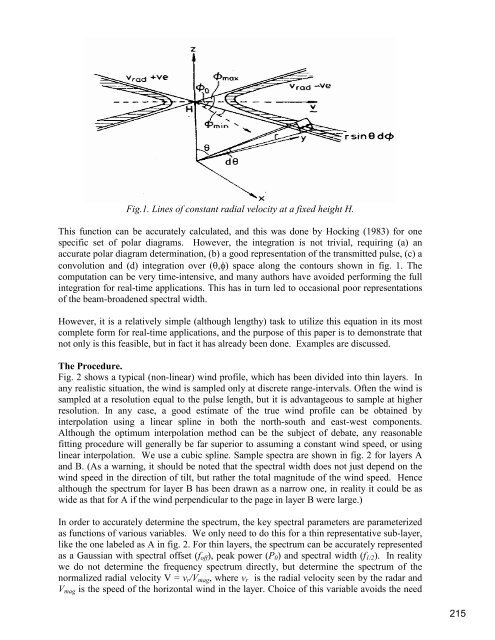
- Page 215 and 216: the beamwidth, α is the zenith ang
- Page 217 and 218: this latitude in late April). Surfa
- Page 219: Fig. 1. Median (upper) winds and (l
- Page 223 and 224: which have not yet been considered
- Page 225 and 226: is calculated from the radiosonde t
- Page 227 and 228: Figure 3: Time-altitude cross-secti
- Page 229 and 230: Absorption of cosmic noise is cause
- Page 231 and 232: Incoherent scatter spectracompared
- Page 233 and 234: variations of spectral widths, refr
- Page 235 and 236: Figure 1. Diurnal variation of Turb
- Page 237 and 238: further experimental test of the ST
- Page 239 and 240: waves can be observed more clearly
- Page 241 and 242: winter and a minimum in summer near
- Page 243 and 244: The main recently assumed mechanism
- Page 245 and 246: Figure 2. Statistics of numbers of
- Page 247 and 248: LIDAR OBSERVATIONS OF MIDDLE ATMOSP
- Page 249 and 250: latitudinal dependence of the seaso
- Page 251 and 252: APPLICATION OF THE DUAL-BEAMWIDTH M
- Page 253 and 254: Figure 2: Mean zonal and meridional
- Page 255 and 256: JLKLLK/ILIL6II/G/II/G/LEODFLK/LO/DD
- Page 257 and 258: The monthly diurnal mean of horizon
- Page 259 and 260: Session I.4: Meteorological Phenome
- Page 261 and 262: Integration of the VHF wind profile
- Page 263 and 264: Figure 1 : Map of the Lago Maggiore
- Page 265 and 266: precipitating clouds, the cyclonic
- Page 267 and 268: Eyewall(a)(b)(c)(d)Fig. 3: Radius-h
- Page 269 and 270: as low as 0.55. The Piura 50-MHz ra
- Page 271 and 272:
place features in the profile with
- Page 273 and 274:
• Period 1 (June 1-10): SCCs exis
- Page 275 and 276:
Sumatera occurs by stratiform cloud
- Page 277 and 278:
very interesting to note the double
- Page 279 and 280:
20(a) Convective Region(b) Transiti
- Page 281 and 282:
Typhoon LekimaFig. 2 Typhoon Lekima
- Page 283 and 284:
Fig. 5 Passage of typhoon Hayan on
- Page 285 and 286:
the 50 cm 2 sensor head, enabling t
- Page 287 and 288:
22 June 2000 23:22:23 - 23:24:20 at
- Page 289 and 290:
the time-height section of a convec
- Page 291 and 292:
Thurai, M., T.Iguchi,T. Kozu, J.D.E
- Page 293 and 294:
There are two main mechanisms which
- Page 295 and 296:
Horel, J.D. and Cornejo-Garrido, A.
- Page 297 and 298:
estimating two independent and redu
- Page 299 and 300:
RASS THETA (K) RASS v-component (m/
- Page 301 and 302:
Surface winds usually range from 10
- Page 303 and 304:
weak (maximum of 5 m s -1 ) and the
- Page 305 and 306:
The vertical component from the VTB
- Page 307 and 308:
Figure 8 shows the profile of virtu
- Page 309 and 310:
2 3D ( , ) ( ) ( ) ˆ ( ) ˆp∆ xm
- Page 311 and 312:
presented in Praskovsky et al. (200
- Page 313 and 314:
In Fig. 2 a sketch of a mountain le
- Page 315 and 316:
In Fig. 8 the lamina is aligned on
- Page 317 and 318:
Figure 1: composite day (13 days) o
- Page 319 and 320:
virtual sensible heat fluxes ( Wm-2
- Page 321 and 322:
3. Characteristics of precipitation
- Page 323 and 324:
Fig. 3: Horizontal distribution of
- Page 325 and 326:
3. Results and discussionUHF profil
- Page 327 and 328:
Figure 4. Monthly variation of slop
- Page 329 and 330:
system with two receiving antennae,
- Page 331 and 332:
cycle of precipitation. Figure 3(a)
- Page 333 and 334:
Histogram of Zonal Velocityh=5.13 K
- Page 335 and 336:
5. Summary of results and concludin
- Page 337 and 338:
the two nearby major cities, Chenna
- Page 339 and 340:
Boundary layer height, km32.521.5(a
- Page 341 and 342:
Figure 1:Data from the MST radar at
- Page 343 and 344:
spectral processing. In this partic
- Page 345 and 346:
3. Results and discussionIn the pre
- Page 347 and 348:
4. SummaryAn attempt has been made
- Page 349 and 350:
The purpose of this study is to exa
- Page 351 and 352:
Figure1. Three-day average of momen
- Page 353 and 354:
3. The improved method to estimate
- Page 355 and 356:
But in case of period until 1800 UT
- Page 357 and 358:
Session I.5: Operational Aspects an
- Page 359 and 360:
The profilers of WINDAS weredesigne
- Page 361 and 362:
NOAA, 1994 : Wind profiler assessme
- Page 363 and 364:
FIRST RESULTS OF THE BOUNDARY LAYER
- Page 365 and 366:
Figure 3. Pulse Design Diagram to s
- Page 367 and 368:
MOVEABLE UHF/S-BAND PROFILER/DISDRO
- Page 369 and 370:
one-minute Z values determined from
- Page 371 and 372:
TOWARD A MULTISENSOR GROUND BASED R
- Page 373 and 374:
3. Cloud Evolution Case StudyOn the
- Page 375 and 376:
DEVELOPMENT OF A DIGITAL RECEIVER F
- Page 377 and 378:
Experiment 1 Experiment 2IPP 999Km
- Page 379 and 380:
ELECTRONIC DIGITAL BEAMFORMING IMPL
- Page 381 and 382:
The main element of the unit (figur
- Page 383 and 384:
.ON-LINE ADAPTIVE DC-GROUND-CLUTTER
- Page 385 and 386:
esulting in a widening of the bandw
- Page 387 and 388:
ON THE RADIATION EFFICIENCY OF COCO
- Page 389 and 390:
Table 2: Experiment #1 results, Tra
- Page 391 and 392:
A NEW NARROW BEAM MF RADAR AT 3 MHZ
- Page 393 and 394:
Off-zenith beams towards N, S, E, W
- Page 395 and 396:
95ALWIN VHF radar: signal powerdB80
- Page 397 and 398:
ANTENNA BEAM VERIFICATION USING COS
- Page 399 and 400:
Figure 2: A 45 MHz reference sky te
- Page 401 and 402:
AN ATTEMPT TO CALIBRATE THE UHF STR
- Page 403 and 404:
is at 4.7 km, but in the first 4-ga
- Page 405 and 406:
QUALITY CONTROL FOR DOPPLER WIND PR
- Page 407 and 408:
The resulting moments are subjected
- Page 409 and 410:
SOUSY RADAR AT JICAMARCA: SYSTEM DE
- Page 411 and 412:
NEControl andcomputer roomCompCoute
- Page 413 and 414:
THE EQUATORIAL ATMOSPHERE RADAR:SYS
- Page 415 and 416:
Table 1: Specifications of the EAR
- Page 417 and 418:
VHF ATMOSPHERIC AND METEOR RADAR IN
- Page 419 and 420:
ased upon a geotechnical engineerin
- Page 421 and 422:
VORTICAL MOTIONS OBSERVED WITH THE
- Page 423 and 424:
interpolation from the original gri
- Page 425 and 426:
A NEW MINIRADAR TO INVESTIGATE URBA
- Page 427 and 428:
e eliminated to analyze correctly t
- Page 429 and 430:
Session PWG 1: System Calibrations
- Page 431 and 432:
Session PWG 2: Data Analysis, Valid
- Page 433 and 434:
• the time series vectors x(k) of
- Page 435 and 436:
Fig. 4: reflectivity of the hydrome
- Page 437 and 438:
Session PWG 3: Accuracies and Requi
- Page 439 and 440:
Session PWG 4: International Collab
- Page 441 and 442:
Session II.E: NOVEL PERSPECTIVES AN
- Page 443 and 444:
2 Proposed AlgorithmReceived signal
- Page 445 and 446:
N#4E-1-16E1A1#1#2A-1-1C1#3C-1-19Fig
- Page 447 and 448:
of conventional DCMP, with which th
- Page 449 and 450:
applying the directional constraint
- Page 451 and 452:
while for a beam of finite width, t
- Page 453 and 454:
In order to make the process more q
- Page 455 and 456:
WHAT IS TURBULENCE SEEN BY VHF RADA
- Page 457 and 458:
Enhanced resolution applyingpulse s
- Page 459 and 460:
Beckmann, Spizichino, 1964Fig. 8 Po
- Page 461 and 462:
Fig. 11 Plots of temporal variation
- Page 463 and 464:
Fig. 14 Distributions of phase cent
- Page 465 and 466:
Hocking, W.K., Radar studies of sma
- Page 467 and 468:
THE STRUCTURE FUNCTION-BASED APPROA
- Page 469 and 470:
{ Ui( t), Vi( t), Wi( t)} = { Ui ,
- Page 471 and 472:
161). Assumption 2H: the instantane
- Page 473 and 474:
Only the second order SF are consid
- Page 475 and 476:
fluctuations umk( t ) along the bas
- Page 477 and 478:
VHF PARASITIC RADAR INTERFEROMETRYF
- Page 479 and 480:
• All the costs of transmitter pr
- Page 481 and 482:
Figure 2: Example of range-azimuth
- Page 483 and 484:
Target Altitude, km1009080706050403
- Page 485 and 486:
ReferencesGriffiths, H. D., A. J. G
- Page 487 and 488:
Participants ListAvery, James P.Uni
- Page 489 and 490:
Hysell, David L.EAS/Cornell Univers
- Page 491 and 492:
Silva, Robert R.ATRADAustraliarsilv
- Page 493 and 494:
AAdachi, A. .......................
- Page 495:
TTabary, P. .......................